Environmental Toxicology, an open online textbook

Environmental Toxicology, an open online textbook

Environmental Toxicology – open online textbook

Developments in Environmental Toxicology: Interview with two pioneers

Developments in Environmental Toxicology: interview with two pioneers

Editors

Cornelis A.M. van Gestel, Frank G.A.J. Van Belleghem, Nico W. van den Brink, Steven T.J. Droge, Timo Hamers, Joop L.M. Hermens, Michiel H.S. Kraak, Ansje J. Löhr, John R. Parsons, Ad M.J. Ragas, Nico M. van Straalen, and Martina G. Vijver

Preface

This open online textbook on Environmental Toxicology aims at covering the field in its full width, including aspects of environmental chemistry, ecotoxicology, toxicology and risk assessment. With that, it will contribute to improving the quality, continuity and transparency of the education in environmental toxicology. We also want to make sure that fundamental insights on fate and effects of chemicals gained in the past are combined with recent approaches of effect assessment and molecular analysis of mechanisms causing toxicity.

The book consists of six chapters, with each chapter being divided into several sub-chapters to enable covering all aspects relevant to the topic. All chapters are designed in a modular way, which each module having clear training goals and being flagged with a number of keywords. Most modules have an average length of 1000-2000 words, a limited number of references, and 3-5 figures and/or tables. A few modules are enlighted with short clips, animations or movies to allow better illustration of the theory. The introduction chapter of the book, for instance, contains a short interview with two key experts reflecting on the development of the field over the past 30 years.

The book contains tools for self-study and training, like a (limited) number of questions at the end of each module. For the future we foresee the addition of separate exercises and other tools that may help the student in understanding the theory.

The development of this open online textbook was carried out by a project team that included a team of editors and some supporting staff. The team of editors consisted of environmental toxicologists and chemists from six Dutch universities. They drafted the outline of the book, assigned leaders for each chapter, and identified authors for each module. Each module is authored by 1-2 members of the project team. When a topic required expertise not present among the project team, an external expert was asked to write a module (see List of authors).

To guarantee quality of the book, each module was reviewed by at least one of the members of the project team but also by an international reviewer from outside the project team (see List of reviewers). An advisory board and a steering committee were involved in supervising the project, as well as educational advisors, while the project team served as an editorial board.

The supporting staff included an expert from the university library of the Vrije Universiteit Amsterdam, who advised on the choice of and working with online publication formats, copyright issues, options for including links to other freely available online materials, etc. We also had support from a designer and a professional drawer, who both contributed to the development of the book.

The publication of this book on an open online publication platform allowing free access to anyone, and facilitates its embedding in Learning Management Systems like Canvas and Blackboard often used in university teaching, so giving students easy access.

The modular composition of the book will allow teachers to design their ‘own’ book, by selecting those modules relevant for the class to teach. This will support flexible use of the book.

The publication as an open online book will allow continuous updating of the book, so to stay on top of new developments in the field. As it stands, about 100 modules have been finalized, another 30 modules are already available in drafs that currently are in the process of reviewing, and some more modules are still in preparation. In spite of this large number of modules, which do provide a good basis for teaching at the BSc level, we do realize the book still is not complete. More advance modules that would facilitate teachign at the MSc and higher level as well as widening the number of topics seems desirable, but such was not possible within the current project. We therefore will continu working on the book, but we also welcome any suggestions for extending the book, and we invite colleagues in environmental toxicology and chemistry to take the initiative to write modules on topics still missing.

The preparation of this book was sponsored by the Netherlands Ministry of Education, Culture and Science through SURF, but could not have been realized without the help of many colleagues who assisted in the writing and reviewing the different modules (see Acknowledgement).


Amsterdam, September 2019

Chapter 1: Environmental toxicology

If you want to re-use this chapter, for e.g. in your electronic learning environment, feel free to copy this url: maken.wikiwijs.nl/120137/1__Introduction

1.1. Environmental toxicology

If you want to re-use this chapter, for e.g. in your electronic learning environment, feel free to copy this url: maken.wikiwijs.nl/120137/1__Introduction


Author: Ad Ragas

Reviewers: Kees van Gestel, Nico van Straalen


Learning objectives

You should be able to

  • characterize the field of environmental toxicology;
  • explain what type of knowledge from environmental chemistry, toxicology and ecology is relevant for environmental toxicology;
  • explain the difference between environmental toxicology and ecotoxicology.


Keywords: Environmental toxicology, environmental chemistry, toxicology, ecology, ecotoxicology


Environmental toxicology is the science that studies the fate and effects of potentially hazardous chemicals in the environment. It is a multidisciplinary field assimilating and building upon knowledge, concepts and techniques from other disciplines, such as toxicology, analytical chemistry, biochemistry, genetics, ecology and pathology. Environmental toxicology emerged in response to the growing awareness in the second part of the 20th century that chemicals emitted to the environment can trigger hazardous effects in organisms living in this environment, including humans. Section 1.3 gives a brief summary of the history of environmental toxicology.


One way to depict the field of environmental toxicology is by a triangle consisting of chemicals, the environment and organisms (Figure 1). The triangle illustrates that the fate and potential hazardous effects of chemicals emitted to the environment are determined by the interactions between these chemicals, the environment and organisms. The fate of substances in the environment is the topic of environmental chemistry, the effects of substances on living organisms is studied by toxicology, and the implications of these effects on higher levels of biological organization are analyzed by the field of ecology.


Another term widely used to refer to this field of study is ecotoxicology. The main distinction is the inclusion of human health as an endpoint in environmental toxicology, whereas ecotoxicology is restricted to ecological endpoints. Since the current book includes human health as an assessment endpoint for environmental contaminants, the term environmental toxicology is preferred over ecotoxicology.


Figure 1: Environmental toxicology studies the interactions between chemicals, organisms and the environment making use of environmental chemistry, toxicology and ecology. Source: Ad Ragas.


Environmental chemists study the fate of chemicals in the environment, e.g. their distribution over different environmental compartments and how this distribution is influenced by the physicochemical properties of a chemical and the characteristics of the environment. They aim to understand the pathways and processes involved in the environmental fate of a chemical after it has been emitted to the environment, including processes such as advection, deposition and (bio)degradation. Within the context of environmental toxicology, the ultimate aim is to produce a reliable assessment of the exposure of organisms, an aim which is often complicated by the enormous heterogeneity of the environment.

Environmental chemists use a variety of tools to analyze and assess the fate of chemicals in the environment. Two fundamental tools are analytical measurements and mathematical modelling. Measurements are essential to acquire new knowledge and insight into the behavior of chemicals in the environment., e.g. measurements on emissions, environmental concentrations and specific processes such as biodegradation. These measurements are analyzed to discover patterns, e.g. between substance properties and environmental characteristics. Once revealed, such patterns can be integrated into a comprehensive mathematical model to predict the fate of and exposure to substances in the environment. If sufficiently validated, these models can subsequently be used by risk assessors to assess the exposure of organisms to chemicals, reducing the need for expensive measurements.

Chapter 2 focuses on the types of chemicals occurring in the environment, their sources and the concentrations found at contaminated sites. In Chapter 3, focus will be on the fate and transport of these chemicals, including aspects of bioavailability and bioaccumulation in organisms.


Toxicologists study the effects of chemicals on organisms, often at the individual level. Fundamental toxicologists aim to understand the mechanisms involved in the toxicity of a compound, whereas more applied toxicologists are primarily interested in the relationship between exposure and effect, often with the aim of identifying an exposure level that can be considered safe. Within this context, the dose concept as introduced by Parcelsus at the start of the 16th century is essential (see Section 1.3), i.e. the likelihood of adverse effects depends on the dose organisms are being exposed to.

The processes taking place after exposure of an organism to a toxicant are often divided into toxicokinetic and toxicodynamic processes. Toxicokinetic processes are those that describe the fate of the toxicant in the organism, including processes such as absorption, distribution, metabolism and excretion (ADME). These toxicokinetic or ADME processes are sometimes collectively referred to as “What the body does to the substance” and determine the exposure level at the site of toxic action, or internal dose. Toxicodynamic processes are those that describe the evolution of an adverse effect from the moment that the toxicant, or one of its metabolites, interacts with a molecular receptor in the body. This interaction is often referred to as the primary lesion or molecular initiating event (MIE). Toxicodynamic processes are sometimes collectively referred to as “What the substance does to the body” and the chain of events leading to an adverse outcome as the adverse outcome pathway (AOP).

The toxicity of a compound thus depends on toxicokinetic as well as toxicodynamic processes. Traditionally, this toxicity is being determined by exposing whole organisms in the laboratory to the substance of interest, and subsequently monitoring the health status of these organisms. However, as a result of the growing societal pressure to reduce animal testing, as well as the increased mechanistic understanding and improved molecular techniques, this so-called “black box approach” is more and more being replaced by a combination of in vitro toxicity testing and “in silico” predictive approaches. Physiologically-based toxicokinetic (PBTK) models are increasingly used to model the fate of chemicals in the body, resulting in a prediction of the internal exposure. In vitro tests and advanced molecular techniques at the gene (genomics) or protein (proteomics)  level may subsequently be used to determine whether these internal exposure levels will trigger adverse effects, although many challenges remain in the prediction of adverse effects based on in vitro test and omics information. Chapter 4 focuses on dose-response relationships, modes of action, species differences in sensitivity and resistance against toxicants.


Ecologists study the interactions between organisms and their environment. Ecology is an important pillar of environmental toxicology, because ecological knowledge is needed to translate effects at the individual level to the ecosystem level; an important endpoint of ecological risk assessments. Such a translation requires specific knowledge, e.g. on life cycles of organisms, natural factors regulating their populations, genetic variability within populations, spatial distribution patterns, and the role organisms play in processes like nutrient cycling and decomposition. Effects considered relevant at the individual level, such as a tumor risk, may turn out to be irrelevant at the population or ecosystem level. Similarly, subtle effects at the individual level may turn out to be highly relevant at the ecosystem level, e.g. behavioral changes after environmental exposure to antidepressants which may affect the population dynamics of fish species. In recent years, there is an increasing interest for the role of the landscape configuration, distribution patterns and their dynamics in environmental toxicology. The spatial configuration of the landscape, the distribution of species and the timing of exposure events turn out to be important determinants of ecosystem effects. The ecological aspects of environmental toxicology will be discussed in Chapter 5.

1.2. DPSIR

Author: Ad Ragas

Reviewers: Frank van Belleghem


Learning objectives

You should be able to:

  • list and describe the five categories of DPSIR;
  • structure a simple environmental problem using the DPSIR framework;
  • describe the position and role of environmental toxicology within the DPSIR framework;
  • indicate the most important advantages and disadvantages of the DPSIR framework.


Keywords: Drivers, pressures, state variables, impacts, responses


On the one hand, environmental toxicology is rooted in more fundamental scientific disciplines like biology and chemistry where curiosity is an important driver for gathering new knowledge. On the other hand, environmental toxicology is a problem-oriented discipline. As such, it is part of the broader field of environmental sciences which analyses the interactions between society and its physical environment in order to promote sustainability. Within this context, knowledge about the interactions of substances with the biotic and abiotic environment is being generated with the ultimate aim to prevent and address potential pollution problems in society. To be able to contribute optimally, an environmental toxicologist should know how pollution problems are structured and what the role of environmental toxicologists is in analysing, preventing and solving such problems. A widely used framework for structuring environmental problems is DPSIR. DPSIR stands for Drivers, Pressures, State, Impacts and Responses (Figure 1). The aim of the current section is to explain the DPSIR framework.


Communication tool

Communication is essential when analysing and addressing societal issues such as environmental pollution. As an environmental toxicologist, you will have to communicate with fellow scientists to develop a common understanding of the pollution problem, and with policy makers and stakeholders (e.g., producers of chemicals and consumers that are being exposed to chemicals)  to explain the scientific state of the art. It is likely that you will use terms like “cause”, “source” and “effects”. However, not everybody will use and perceive these terms in the same way. Some people may argue that a farmer is the main cause of pesticide pollution, whereas others may argue that it is the pesticide manufacturer, or even the increasing world population. Likewise, some people may perceive the concentration of pesticides in water as an effect of pesticide use, whereas others may refer to the extinction of species when talking about effects. These differences may result in miscommunication, complicating scientific analysis and the search for appropriate solutions.

The DPSIR framework is a tool that helps preventing such communication problems. It provides a common and flexible frame of reference to structure environmental issues by describing these in terms of drivers, pressures, state (variables), impacts and responses (Figure 1). Flexibility is an important characteristic of the framework, enabling adaptation to the problem at hand. The DPSIR framework should not be considered a panacea or used as a mould that rigidly fits all environmental issues. Its main strength is that it stimulates communication between scientists, policy makers and other actors and thereby supports the development of a common understanding.


Figure 1. The DPSIR framework is a tool to structure environmental issues by organizing the processes in Drivers, Pressures, State (variables), Impacts and Responses. Source: Ad Ragas.


The framework

The DPSIR framework essentially is a cause-and-effect chain that aims to capture the main processes involved in an environmental issue; from its origin to the changes it triggers in the environment and in society. These processes are organized in five main categories, i.e.:

  • are the human needs underlying the human activities that ultimately result in adverse effects. An example is the human need for food resulting in the use of pesticides such as neonicotinoids.
  • are human activities initiated to fulfil human needs and resulting in changes in the physical environment that ultimately lead to - often unforeseen – adverse consequences for the environment or certain groups of society that are perceived as problematic, either now or in the future. An example is the use of neonicotinoids in agriculture.
  • refers to the status of the physical environment. The state of the environment is often quantified using observable changes in environment parameters, e.g., the concentration of neonicotinoids in water, air, soil and biota.
  • are any changes in the physical environment or society that are a consequence of the environmental pressures and that are perceived as problematic by society or some groups in society. An example is the increasing bee mortality that is, at least partly, attributed to the use of neonicotinoids. Or the human health effects of pesticides.
  • are all initiatives developed by society to address the issue. These can range from gathering knowledge to developing policy plans and taking measures to mitigate effects or reduce emissions. Examples include the introduction of a risk-based admission procedure for neonicotinoids, the introduction of more efficient spraying techniques, and the development of environmentally friendly pest control techniques.


In principle, any environmental issue can be captured in a DPSIR. But it is important to realize that the labelling of processes as either drivers, pressures, state (variables), impacts or responses is likely to differ between people since the categories are broadly defined and the level of detail in the processes considered may vary. For example, some people may argue that “agriculture” should be classified as a driver, whereas others may argue it is a pressure. Yet other people may deal with this issue by adapting the DPSIR framework, i.e. by adding a new category called “human activities” that is placed in-between the drivers and the pressures. Another typical issue is the labelling of consecutive changes in the physical environment such as rising CO2 levels, increases in temperature and changes in species abundance. These changes can be labelled as changes in consecutive state variables, i.e. state variables of 1st, 2nd and 3rd order. The idea is that 1st order changes trigger 2nd order changes, e.g. rising CO2 levels triggering a rise in temperature, and 2nd order changes trigger 3rd order changes, in this case a shift in species abundance. The change in species abundance may also be labelled as an impact, provided this change is perceived as problematic by (groups in) society. The category “impacts” is closely related to the protection goals of risk assessment (see the Section Ecosystem services and protection goals). If there is consensus in society that an impact should be prevented, it becomes a protection goal. All these examples illustrate that the DPSIR framework should be applied in a flexible way and that communication is essential.

Environmental toxicology mainly focuses on the Pressures, State and Impacts blocks of the DPSIR chain. The use of chemicals by society, e.g. in agriculture or in consumer products, and their emission to the environment belongs to the Pressure block. The fate of chemicals in the environment and their accumulation in organisms belongs to the State block. And the adverse effects triggered in ecosystems and humans belong to the Impact block. An important step in risk assessment of chemicals (Chapter 6) is the derivation of safe exposure levels such as the Predicted No Effect Concentration (PNEC) for ecosystems or the Acceptable Daily Intake (ADI) for humans. In terms of DPSIR, this boils down to defining an acceptable impact level (e.g. a zero effect level or a 1 in a million tumor risk) and translating this into a corresponding state parameter (e.g. the chemical concentration in air or water). Fate modelling (Section on Modelling exposure) aims to predict soil, water, air and organisms (all State parameters) based on emission data (a Pressure parameter).


Figure 2. The extended DPSIR framework to put more emphasis on the societal dimension, i.e. governance, awareness, resources and knowledge. Source: Ad Ragas.


The DPSIR framework has been criticized because it tries to capture all processes in cause-and-effect relationships, resulting in a bias towards the physical dimension of environmental issues, e.g. human activities, emissions, physical effects and mitigations measures. The societal dimension is less easily captured, e.g. knowledge generation, governance structures, resources needed to implement measures, awareness and societal framing of the problem (Svarstad et al., 2008). Although the DPSIR framework can been adapted to accommodate some of these aspects (e.g., see Figure 2), it should be acknowledged that it has its limitations. Several alternative frameworks have been developed, and some of these better capture the societal dimension (Gari et al., 2015; Elliott et al., 2017). Nevertheless, DPSIR can be a useful framework to contextualize the problems that are addressed in environmental toxicology. It nicely shows why knowledge on the fate and impact of chemicals (state and impacts) is needed to address pollution issues and that the use of this knowledge is always subject to valuation, i.e. it depends on how society values the adverse effects triggered by the pollution. DPSIR is also widely used by national and international institutes such as the European Environment Agency (EEA), the United States Environmental Protection Agency (US-EPA) and the Organisation for Economic Cooperation and Development (OECD). The DPSIR framework is sometimes also used as a first step in modelling, especially its physical dimension. Once relevant processes have been identified, these are then described quantitatively resulting in models that can be used to predict environmental concentrations or ecological effects of substances based on knowledge about human activities or emissions.


References

Gari, S.R., Newton, A., Icely, J.D. (2015). A review of the application and evolution of the DPSIR framework with an emphasis on coastal social-ecological systems. Ocean & Coastal Management 103, 63-77.

Svarstad, H., Petersen, L.K., Rothman, D., Siepel, H., Wätzold, F. (2008). Discursive biases of the environmental research framework DPSIR. Land Use Policy 25, 116–125.

Elliott, M., Burdon, D., Atkins, J.P., Borja, A., Cormier, R., de Jonge, V.N., Turner, R.K. (2017). “And DPSIR begat DAPSI(W)R(M)!” - A unifying framework for marine environmental management. Marine Pollution Bulletin 118, 27–40.

1.3. Short history

Author: Ansje Löhr

Reviewers: Ad Ragas, Kees van Gestel, Nico van Straalen


Learning Objective:

You should be able to

  • summarize the history of environmental toxicology
  • describe the increasing awareness over time of environmental and health risks


Keywords: Paracelsus; Rachel Carson (Silent Spring); Awareness; SETAC; standards


History

From earliest times, man has been confronted with the poisonous properties of certain plants and animals. Poisonous substances are indeed common in nature. People who still live in close contact with nature generally possess an extensive empirical knowledge of poisonous animals and plants. Poisons were, and still are, used by these people for a wide range of applications (catching fish, poisoning arrowheads, in magic rituals and medicines). The first Egyptian medical documentation (written in the Ebers Papyrus) dates from 1550 BC and demonstrates that the ancient Egyptians had an extensive knowledge of the toxic and curative properties of natural products. A good deal is known about the information regarding toxic substances possessed by the Greeks and the Romans. They were very interested in poisons and used them to carry out executions. Socrates, for example, was executed using an extract of hemlock (Conium maculatum). It was also not unusual to use a poison to murder political opponents. Poisons were ideal for that purpose, since it was usually impossible to establish the cause of death by examining the victim. To do so would have required advanced chemical analysis, which was not available at that time.

Early European literature also includes a considerable number of writings on toxins, including the so-called herbals, such as the Dutch “Herbarium of Kruidtboeck” by Petrus Nylandt dating from 1673. Poisoning sometimes assumed the character of a true environmental disaster. One example is poisoning by the fungus Claviceps purpurea, which occurs as a parasite in grain, particularly in rye (spurred rye) and causes the condition known as ergotism. In the past, this type of epidemic has killed thousands of people, who ingested the fungus with their bread. There are detailed accounts of such calamities. For example, in the year 992 an estimated 40,000 people died of ergotism in France and Spain. People were not aware of the fact that death was caused by eating contaminated bread. It was not until much later that it came to be understood that large-scale cultivation of grain involved this kind of risk.


Paracelsus

It was pointed out centuries ago that workers in the mining industry, who came into contact with a variety of metals and other elements, tended to develop specific diseases. The symptoms regularly observed as a result of contact with arsenic and mercury in the mining industry were described in detail by the famous Swiss physician Paracelsus (Figure 1) in his 1567 treatise “Von der Bergsucht und anderen Nergkrankheiten” (miners sickness and other diseases of mining). During the emergence of the scientific renaissance of the 16th century, Paracelsus (1493 - 1541) drew attention to the dose-dependency of the toxic effect of substances. In the words of Paracelsus, “all Ding sind Gifft … allein die Dosis macht das ein Ding kein Gifft is” (everything is a poison … it is only the dose that makes it not a poison). This principle is just as valid today. At the same time, it is one of the most neglected principles in the public understanding of toxicology.


Figure 1: A portrait of Paracelsus (PORTRAIT PRESUME DU MEDECIN PARACELSE (1493-1541) (Source: https://commons.wikimedia.org/wiki/File:Paracelsus.jpg)


A work from the same period “De Re Metallica” by Gergius Agricola (Georg Bauer, 1556), deals with the health aspects of working with metals. Agricola even advised preventive aspects, such as wearing protective clothing (masks) and using ventilation.


Scrotum cancer in chimney sweepers: carcinogenicity of occupational exposure

Another example of the rising awareness of the effects of poisons on human health came with the suggestion, by Percival Pott in 1775, that the high frequency of scrotum cancer among British chimney sweepers was due to exposure to soot. He was the first to describe occupational cancer.


A part of the essay by Percival Pott “The fate of these people seems singularly hard; in their early infancy, they are most frequently treated with great brutality, and almost starved with cold and hunger; they are thrust up narrow, and sometimes hot chimnies, where they are bruised, burned, and almost suffocated; and when they get to puberty, become peculiarly liable to a most noisome, painful, and fatal disease.” See the rest of the original text of his essay here.


Soot consists of polycyclic aromatic hydrocarbons (PAHs) and their derivatives. The exposure to soot came with concurrent exposure to a number of carcinogens such as cadmium and chromium. From the 1487 cases of scrotal cancer reported, 6.9 % occurred in chimney sweepers. Scrotal and other skin cancers among chimney sweepers were at the same time also reported from several other countries.


Peppered moth in polluted areas

Changes in the environment due to environmental pollution led to interesting insights in the potential of species to adapt for survival and the role of natural selection in it. A famous example of such micro-evolution is the peppered moth, Biston betularia, that is generally a mottled light color with black speckles. This pattern gives them good camouflage against lichen-covered tree trunks while resting during the day. During the industrial revolution, the massive increase in the burning of coal resulted in the emission of dark smoke turning the light trees in the surrounding areas dark. As a consequence, the dark, melanic form of the peppered moth took over in industrial parts of the United Kingdom during the 1800s. The melanic forms used to be quite rare, but their dark color served as a protective camouflage from bird populations in the polluted areas. This allowed them to become dominant in areas with soot-covered trunks. Two British biologists, Cedric Clarke and Phillip Sheppard, discovered this when they pinned dead moths of the two types on dark and light backgrounds to study their predation by birds. The dark moths had an advantage in the dark forests, a result of natural selection. In areas where air pollution has decreased the melanic form became less abundant again.  


Video on peppered moths


Awareness in the 1950s and 1960s

After the second world war, synthetic chemical production became widespread. However, there was limited awareness of the environmental and health risks. In the 1950s, Environmental Toxicology came to light as a result of increasing concern about the impact of toxic chemicals on the environment. This led toxicology to expand from the study of the toxic impacts of chemicals on man to that of toxic impacts on the environment. An important person in raising this awareness was Rachel Carson. Her book “Silent Spring”, published in 1962, in which she warned of the dangers of chemical pesticides, triggered widespread public concern on the dangers of improper pesticide use.


First have a look at an historical clip on the use of dichlorodiphenyltrichloroethane, commonly known as DDT, that was developed in the 1940s as the first modern synthetic insecticide.


Silent Spring – Rachel Carson  


DDT is very persistent and tends to concentrate when moving through the food chain. As a consequence, the use of DDT led to very high levels, especially in organisms high in the food chain. Bioaccumulation in birds appeared to cause eggshell thinning and reproductive failure. Because of the increasing evidence of DDT's declining benefits and its environmental and toxicological effects, the United States Department of Agriculture, the federal agency responsible for regulating pesticide use, began regulatory actions in the late 1950s and 1960s to prohibit many of its uses. By the 1980s, the use of DDT was also banned from most Western countries.


Large environmental disasters

As a result of large environmental disasters, awareness amongst the general public increased. An enormous industrial pesticide disaster occurred in 1984 in Bhopal, India, when more than 40 ton of the highly toxic methyl isocyanate (MIC) gas leaked from a pesticide plant into the towns located near the plant. Almost 4000 people were killed immediately and 500,000 people were exposed to the poisonous substance causing many additional deaths because of gas-related diseases. The plant was actually initially only allowed to import MIC but was producing it on a large scale by the time of the disaster and safety procedures were far below (international) standards for environmental safety. The disaster made it very clear that this should be changed to avoid other large-scale industrial disasters.

The Sandoz agrochemical spill close to Basel in Switzerland in 1986 was the result of a fire in a storehouse. The emission of large amounts of pesticide caused severe ecological damage to the Rhine river and massive mortality of benthic organisms and fish, particularly eels and salmonids.

At the time of these incidents, environmental standards for chemicals were still largely lacking. The incidents triggered scientists to do more research on the adverse environmental impacts of chemicals. Public pressure to control chemical pollution increased and policy makers introduced instruments to better control the pollution, e.g. environmental permitting, discharge limits and environmental quality standards.


Our Common Future

In 1987, the World Commission on Environment and Development released the report “Our Common Future”, also known as the Brundtland Report. This report placed environmental issues firmly on the political agenda, defining sustainable development as “a development that meets the needs of the present without compromising the ability of future generations to meet their own needs”. Another influential book was “Our stolen future” written by Theo Colborn and colleagues in 1996. It raised awareness of the endocrine disrupting effects of chemicals released into the environment and threatening (human) reproduction by emphasizing it not only concerns feminization of fish or other organisms in the environment, but also the human species.


Please watch the video “Developments in Environmental Toxicology - Interview with two pioneers” included at the start of the Introduction of this book.


SETAC

Before the 1980s, no forum existed for interdisciplinary communication among environmental scientists —biologists, chemists, toxicologists— as well as managers and others interested in environmental issues. The Society of Environmental Toxicology and Chemistry (SETAC) was founded in North America in 1979 to fill this void. In 1991, the European branch started its activities and later SETAC also established branches in other geographical units, like South America, Africa and South-East Asia. SETAC publishes two journals: Environmental Toxicology and Chemistry (ET&C) and Integrated Environmental Assessment and Management (IEAM). SETAC also is active in providing training, e.g. a variety of online courses where you can acquire skills and insights in the latest developments in the field of environmental toxicology. Based on the growth in the society’s membership, the meeting attendance and their publications, a forum like SETAC was clearly needed. Read more on SETAC, their publications and how you can get involved here.

Where SETAC focuses on environmental toxicology, international toxicological societies have also been established like EUROTOX in Europe and the Society of Toxicology (SOT) in North America. In addition to SETAC, EUROTOX and SOT, many national toxicological societies and ecotoxicological counterparts or branches became active since the 1970s, showing that environmental toxicology has become a mature field of science. One element indicative of this maturation, also is that the different societies have developed programmes for the certification of toxicologists.


References

Carson, R. (1962). Silent Spring. Houghton Mifflin Company.

Colborn, T., Dumanoski, D., Peterson Myers, J. (1996). Our Stolen Future: Are We Threatening Our Fertility, Intelligence, and Survival? A Scientific Detective Story. New York: Dutton. 306 p.

World Commission on Environment and Development (1987). Our Common Future. Oxford: Oxford University Press. p.27.


Chapter 2: Environmental Chemistry, Chemicals

If you want to re-use this chapter, for e.g. in your electronic learning environment, feel free to copy this url: maken.wikiwijs.nl/120172/2__Environmental_Chemistry___Chemicals

2.1. Introduction

Authors: John Parsons, Steven Droge

Reviewer: Kees van Gestel


Leaning objectives:

You should be able to:

  • mention the main groups of environmental pollutants
  • comprehend the molecular structures of the most important organic pollutants
  • mention the most important functional groups determining the environmental properties of organic pollutants


Keywords: natural toxicants, molecular structures, pollutant classes, anthropogenic pollutants


Introduction

Environmental toxicology deals with the negative effects of the exposure to chemicals we regard as pollutants (or contaminants/toxicants). Environmental toxicants receive a lot of media attention, but many critical details are getting lost or are easily forgotten. The clip "You, Me, DDT" shows the discovery of the grandson of the works of his grandfather, the Swiss inventor of the insecticide DDT, Paul Hermann Müller, who received the Nobel Prize for Medicine for that in 1948 (see also Section 1.3). The clip "Stop the POPs" interviews (seemingly) common people about one of the most heavily regulated group of pollutants.

Organisms, including humans, have always been exposed to chemicals in the environment and rely on many of these chemicals as nutrients. Volcanoes, flooding of acid sulfur lakes, and forest fires have caused widespread contamination episodes. Organisms are also in many cases directly or indirectly involved in the fate and distribution of undesirable chemicals in the environment. Many naturally occurring chemicals are toxicants already (see also Section 1.3), think for example about:

  • local arsenic or mercury hotspots in the Earth’s crust, contaminating water pumps or rice irrigation fields;
  • plant-based defence chemicals such as alkaloids, morphine in poppy seeds, juglone from black walnut trees);
  • fungal toxins, such as mycotoxins threatening grain storage depots after harvests;
  • bacterial toxins, such as the botulinum toxin, a neurotoxic protein produced by the bacterium Clostridium botulinum which is the most acutely lethal toxin known at ~10 ng/kg body weight when inhaled;
  • phycotoxins, produced by algae, in mass algal blooms or those that may end up at dangerous levels in shell food;
  • zootoxins in animals, such as venom of snakes and defensive toxins on the skin of amphibians.

Human activities have had an enormous impact on the increased exposure to natural chemicals as a result of, for example, the mining and use of metals, salts and fossil fuels from geological resources. This is for example the case for many metals, nutrients such as nitrate, and organic chemicals present in fossil fuels. Additionally, the industrial synthesis and use of organic chemicals, and the disposal of wastes, have resulted in a wide variety of hazardous chemicals that had either never existed before, or at least not in the levels or chemical form that occur nowadays in our heavily polluted global system. These are typically organic chemicals that are referred to as anthropogenic (`due to humans in nature´) or xenobiotic (`foreign to organisms´) chemicals. In this chapter we aim to clarify the key properties and functionalities of the most common groups of pollutants as a result from human activities, and provide some background on how we can group them and understand their behaviour in the environment.

In the field of environmental toxicology, we are most often concerned about the effects of two distinct types of contaminants: metals and organic chemicals. In some cases other chemicals, such as radioactive elements, may also be important while we could also consider the ecological effects of highly elevated nutrient concentrations  (eutrophication) as a form of environmental toxicology.


Metals

Metals and metalloids (elements intermediate between metals and non-metals) comprise the majority of the known elements. They are mined from minerals and used in an enormous variety of applications either in their elemental form or as chemicals with inorganic or organic elements or ions. Many metals occur as cations, but many processes influence the dissolved form of metals. Aluminium for example for example is only present under very acidic conditions as dissolved cation (Al3+), while at neutral pH the metal speciates into for example certain hydroxides (Al(OH3)0). Mercury as free ion is present at (Hg2+) but due to microbial transformation the highly toxic product methylmercury (CH3Hg+, or MeHg+) is formed. Mining and processing of metals together with disposal of metal-containing wastes are the main contributors to metal pollution although sometimes metals are introduced deliberately into the environment as biocides. The widely used pesticide copper sulfate in e.g. grape districts is an example (LINK on comparison to glyphosate here). More information on metals considered to be environmental pollutants is given in Section 2.2.1.


Organic chemicals

Organic chemicals are manufactured to be used in a wide variety of applications. These range from chemicals used as pesticides to industrial intermediates, fossil fuel related hydrocarbons, additives used to treat textiles and polymers, such as flame retardants and plasticisers, and household chemicals such as detergents, pharmaceuticals and cosmetics.

Organic chemicals that we regard as environmental pollutants include a huge variety of different structures and have a wide variety of properties that influence environmental distribution and toxicity. With such a wide variety of chemicals to deal with, it is useful to classify them into groups. Depending on our interest, we can base this classification on different aspects, for example on their chemical structure, their physical and chemical properties, the applications the chemicals are used in, or their effects on biological systems. These aspects are of course closely related to their chemical structure as this is the basis of the properties and effects of chemicals. An overview of different ways of classifying environmental contaminant (sometimes referred to as ecotoxicants) is shown in Tables 1A, 1B, and 1C.


Table 1A. Grouping options of organic contaminants with specific chemical structures

Term

Characteristics

Examples

Hydrocarbons

More CHx units: higher hydrophobicity/lipophilicity, and lower aqueous solubility

hexane

Polycyclic aromatic hydrocarbons

Combustion products. Flat structure

naphthalene, B[a]P

Halogenated hydrocarbons

H substituted by fluor, chlorine, bromide, iodine. Often relatively persistent

PCB, DDT, PBDE

Dioxins and furans

Combustion/industrial products, one or two oxygen atoms between two aromatic rings. Highly toxic.

TCDD, TCDF

Organometallics

Organic chemicals containing metals, used e.g. in anti-fouling paints

tributyltin

Organophosphate pesticides

Phosphate esters, often connecting two lipophilic groups. Act on nervous system

chlorpyrifos

Pyrethroids

Usually synthetic pesticides based on natural pyrethrum extracts

fenvalerate

Neonicotinoids

Synthetic insecticides with aromatic nitrogen, related to the alkaloid nicotine

imidacloprid

… Endless varieties / combinations and ...

...too many characteristics to list

...


Table 1B. Grouping options of organic contaminants with specific properties

Term

Characteristics

Examples

Persistent organic pollutants (POPs)

Bioaccumulative, end up even in remote Arctic systems

PCBs, PFOS

Persistent mobile organic chemicals (PMOCs)

Difficult to remove during drinking water production

PFBA, metformin

Ionogenic organic chemicals (IOCs)

Acids or bases, predominantly ionized under environmental pH

Prozac, MDMA, LAS

Substances of unknown or variable composition,  complex reaction products or of biological materials (UVCB)

Multicomponent compositions of often analogue structures with wide ranging properties.

Oil based lubricants

Plastics

Chains of repetitive monomer structures. Wide ranging size/dimensions.

Polyethylene,

silicone, teflon

Nanoparticles (NP)

Mostly manufactured particles with >50% having dimensions ranging 1 - 100 nm.

Titanium dioxide (TiO2), fullerene


Table 1C. Grouping options of organic contaminants with specific usage

Term

Characteristics

Examples

Pesticides

Herbicides

Insecticides

Fungicides

Rodenticides

Biocides

Toxic to pests

Toxic to plants

Toxic to insects

Toxic to fungi

Toxic to rodents

Toxic to many species

DDT

atrazine, glyphosate

Chlorpyrifos, parathion

Phenyl mercury acetate

Hydrogen cyanide

Benzalkonium

Pharmaceuticals

Specifically bioactive chemicals with often (un)known side effects. Many bases.

diclofenac (pain killer), iodixanol (radio-contrast), carbemazepine, prozac

Drugs of abuse

Often opioid based but also synthetic designer drugs with similar activity. Many are are ionogenic bases.

cannabinoids, opioids,

amphetamine, LSD

Veterinary Pharmaceuticals

Can include relatively complex (ionogenic) structures

antibiotics, antifungals, steroids, non-steroidal anti-inflammatories

Industrial Chemicals

Produced in large volumes by chemical industry for a wide array of products and processes

phenol

Fuel products

Flammable chemicals

kerosene

Refrigerants and propellants

Small chemicals with specific boiling points

freon-22

Cosmetics/personal care products

Wide varieties of specific ingredients of formulations that render specific properties of a product

sunscreen, parabenes

Detergents and surfactants

Long hydrophobic hydrocarbon tails and polar/ionic headgroups

Sodium lauryl sulfate (SLS), benzalkonium

Food and Feed Additives


To preserve flavor or enhance its taste, appearance, or other qualities

“E-numbers”, acetic acid = E260 in EU, additive 260 in other countries


Chapter 2 mostly discusses groups of chemicals in separate modules according to the specific environmental properties in Table 1B (Section 2.2) and specific applications in Table 1C (Section 2.3), according to which certain regulations apply in most cases. The property classifications can be based on (often interrelated) properties such as solubility (in water), hydrophobicity (tendency to leave the water), surface activity (tendency to accumulate at surfaces of two phases, such as for “surfactants”), polarity, neutral or ionic chemicals and reactivity. Other classifications very important for environmental toxicology are based on environmental behaviour or effects, such as persistency (“P” increasing problems with increased emissions), bioaccumulation potential (“B”, up-concentration in food chains), or type of specific toxic effects (“T”). The influence of specific chemical structures such as in Table 1A is further clarified in the current introductory chapter in order to better understand the basic chemical terminology.


Structures of organic chemicals and functional groups

  • Hydrocarbons and polycyclic aromatic hydrocarbons

As the name suggest, hydrocarbons contain only carbon and hydrogen atoms and can therefore be considered to be the simplest group of organic molecules. Nevertheless, this group covers a wide variety of aliphatic, cycloaliphatic and aromatic structures (see Figure 1 for some examples) and also a wide range of properties. What this group shares is a low solubility in water with the larger molecules being extremely insoluble and accumulating strongly in organic media such as soil organic matter.


Figure 1. Examples of hydrocarbons.


As a result of the ability of carbon to form strong bonds with itself and other atoms to form structures containing long chains or rings of carbon atoms there is a huge and increasing number (millions) of organic chemicals known. Chemicals containing only carbon and hydrogen are known as hydrocarbons. Aliphatic molecules consist of chains of carbon atoms as either straight or branched chains. Molecules containing multiple carbon-carbon bonds (C=C) are known as unsaturated molecules and can be converted to saturated molecules by addition of hydrogen.

Cyclic alkanes consist of rings or carbon atoms. These may also be unsaturated and a special class of these is known as aromatic hydrocarbons, for example benzene in Figure 1. The specific electronic structure in aromatic molecules such as benzene makes them much more stable than other hydrocarbons. Multiple aromatic rings linked together make perfectly flat molecules, such as pyrene in Figure 1, that can be polarized to some extent because of the shared electron rings. In larger sheets, these polycyclic aromatic molecules also make up the basic graphite structure in pencils, and also typically represent the strongly adsorbing surfaces of black carbon phases such as soot and activated carbon.


The structures of organic chemicals help to determine their properties as behaviour in the environment. At least as important in this regard, however, is the presence of functional groups. These are additional atoms or chemical groups that are present in the molecule that have characteristic chemical effects such as increasing or decreasing solubility in water, giving the chemical acidic or basic properties or other forms of chemical reactivity. The common functional groups are shown in Table 2.


Table 2. Common Functional Groups, where R are carbon backbone or hydrogen units


  • Halogenated hydrocarbons: first generation pesticides

The first organic chemical recognised as an environmental pollutant was the insecticide DDT (see clip 1 at the start of this chapter). It later became clear that other organochlorine pesticides such as lindane and dieldrin (Table 3) were also widely distributed in the environment. This was also the case for polychlorinated biphenyls (PCBs) and other organochlorinated industrial chemicals. These chemicals all share a number of undesirable properties such as environmental persistence, very low solubility in water and high level of accumulation in biota to potentially toxic levels. Many organochlorines can be viewed as hydrocarbons in which hydrogen atoms have been replaced by chlorine. This makes them even less soluble than the corresponding hydrocarbon due to the large size of chlorine atoms. In addition, chlorination also makes the molecules more chemically stable and therefore contributes to their environmental persistence. Other organochlorines contain additional functional groups, such as the ether bridges in PCDDs and PCDFs (better known as dioxins and dibenzofurans) and ester groups in the 2,4-D and 2,4,5-T herbicides. Many organochlorines were applied very successfully in huge quantities as pesticides for decades before their negative effects such as persistence and accumulation in biota became apparent. It is therefore no coincidence that the initial set of Persistent Organic Pollutants (POPs) identified in the Stockholm Treaty (see below) as chemicals that should be banned were all organochlorines, as shown in Table 3.  

As well as chlorine, other halogens such as bromine and fluorine are used in important groups of environmental contaminants. Organobromines are best known as flame retardants and have been applied in large quantities to improve the fire safety of plastics and textiles. They share many of the same undesirable properties of organochlorines and several classes have now been taken out of production. Organofluorines are another important class of halogenated chemicals, and part of the well-known group of ozone depleting CFCs (Section 2.3.6). In particular, per-and polyfluoralkyl substances are widely used as fire-stable surfactants in fire-fighting foams, as grease and water resistant coatings and in the production of fluoropolymers such as Teflon. Organofluorines are much more water soluble and much less bioaccumulative than organochlorines and organobromines but are extremely persistent in the environment.

The recognition of these organochlorines as harmful environmental contaminants eventually resulted in measures to restrict their manufacture and use in the Stockholm Convention on Persistent Organic Pollutants signed in 2001 to eliminate or restrict the production and use of persistent organic pollutants (POPs). This initial list of POPs has been subsequently augmented with other harmful halogenated organic pollutants up to a total of 29 chemicals, which are either to be eliminated, restricted, or required measured to reduce unintentional releases. POPs are further discussed in section 2.2.4.


Table 3. Key persistent organic pollutants, also named POPs – the Dirty Dozen


Additional POPs to eliminate include: chlordecone, lindane (hexachlorocyclohexane), pentachlorobenzene, endosulfan, chlorinated naphthalenes, hexachlorobutadiene, tetrabromodiphenylether, and pentabromodiphenylether decabromodiphenyl ether (BDEs).


  • Alternatives for the organochlorine pesticides: effective functional groups

Since the signing of the Stockholm Convention, organochlorine pesticides have been replaced in most countries by more modern pesticide types such as the organophosphorus and carbamate insecticides. These compounds are less persistent in the environment, but still could pose elevated risks to environments surrounding the agricultural sites, and increased levels on food produced on these agricultural sites. The very toxic organophosphorus neurotoxicant parathion has been in use since the 1940s, and has the typical two lipophilic side chains on two esters (ethyl units), as well as a polar unit. Parathion has caused hundreds of fatal and non-fatal intoxications worldwide and as a result it is banned or restricted in 23 countries. The relatively comparable organophosphate structure of diazinon has been widely used for general-purpose gardening and indoor pest control since the 1970s, but residential use was banned in the U.S. in 2004. In Californian agriculture however, 35000 kg diazinon was used in 2012. The carbamate based insecticide carbaryl is toxic to target insects, and also non-target insects such as bees, but is detoxified and eliminated rapidly in vertebrates, and not secreted in milk. Although illegal in 7 countries, carbaryl is the third-most-used insecticide in the U.S., approved for more than 100 crops. In 2012, 52000 kg carbaryl was used in California, while this was 3 times more in 2000. Neonicotinoid insecticides, with the typical aromatic ring containing nitrogen, form a third generation of pesticide structures. Imidacloprid is currently the most widely used insecticide worldwide, but as of 2018 banned in the EU, along with two other neonicotinoids clothianidin and thiamethoxam.


Figure 2. Some examples of second and third generation replacements of organochlorine pesticides.


  • Relatively simple and (very) complex pollutants

As well as the pesticides discussed above, many other chemicals are brought into the environment inadvertently during their manufacture, distribution and use and the range of chemicals recognised as problematic environmental contaminants has expanded enormously. These include fossil fuel-related hydrocarbons, surfactants, pigments, biocides and chemicals used as pharmaceuticals and personal care products (PPCPs). Figure 3 gives an illustrative overview of the major routes by which PPCPs, but also many other anthropogenic contaminants other than pesticides, are released into the environment. Particularly wastewater treatment systems form the main entry point for many industrial and household products.


Figure 3. Emission pathways to soil and water for pharmaceuticals and personal care products. Adapted from Boxall et al. (2012) by Evelin Karsten-Meessen.


The wide variety of contaminant structures does not mean that most chemicals have become increasingly more complex. For risk assessment, molecular properties such as water solubility, volatility and lipophilicity are often estimated based on quantitative structure-property relationships (Section 3.4.3). With increasingly complex structures, such property-estimations based on the molecular structure become more uncertain.

The antibiotic erythromycin for example (Figure 4), is a very complex chemical structure (C37H67NO13) that has 13 functional units along with a 14 member ring. In addition, the tertiary nitrogen group is an amine base group that can give the molecule a positive charge upon protonation, depending on the environmental pH. Erythromycin is on the World Health Organization's List of Essential Medicines (the most effective and safe medicines needed in a health system), and therefore widely used. Continuous emissions in waste streams pose a potential threat to many ecosystems, but many environmentally and toxicologically relevant properties are scarcely studied, and poorly estimated.


Figure 4. Relatively simple or (very) complex chemicals? Glyphosate speciation profile (chemicalize.org) for the 4 dominant glyphosate different species. Glyphosate in soil (pH4-8) predominantly occurs with 3 charged groups (net charge -1), partly with 4 charged groups (-2). The soap SLS is always negatively charged, GHB predominantly negative (pKa 4.7), amphetamine predominantly positive (pKa 9.9), erythromycin predominantly positive (pKa 8.9)


There are also many contaminants or toxicants with a seemingly simple structure. Many surfactants are simple linear long chain hydrocarbons with a polar or charged headgroup (Figure 4). The illicit drug amphetamine has only a benzene ring and an amine unit, the illicit drug GHB only an alcohol and a carboxylic acid, the herbicide glyphosate only 16 atoms. Still, these 4 chemical examples also have acidic or basic units that often result in predominantly charged organic molecules, which also strongly influences their environmental and toxicological behaviour (see sections on PMOCs and Ionogenic Organic Compounds). In case of glyphosate, the chemical has 4 differently charged forms depending on the pH of the environment. At common pH of 7-9, glyphosate has all charged groups predominantly ionized, making it very difficult to derive calculations on environmental properties.


References

Boxall, A. B. A., Rudd, M. A., Brooks, B. W., Caldwell, D. J., Choi, K., Hickmann, S., Innes, E., Ostapyk, K., Staveley, J. P., Verslycke, T., Ankley, G. T., Beazley, K. F., Belanger, S. E., Berninger, J. P., Carriquiriborde, P., Coors, A., DeLeo, P. C., Dyer, S. D., Ericson, J. F., Gagné, F., Giesy, J. P., Gouin, T., Hallstrom, L., Karlsson, M. V., Larsson, D. G. J., Lazorchak, J. M., Mastrocco, F., McLaughlin, A., McMaster, M. E., Meyerhoff, R. D., Moore, R., Parrott, J. L., Snape, J. R., Murray-Smith, R., Servos, M. R., Sibley, P. K., Oliver Straub, J., Szabo, N. D., Topp, E., Tetreault, G. R., Trudeau, V. L., Van der Kraak, G. (2012). Pharmaceuticals and personal care products in the environment: what are the big questions? Environmental Health Perspectives 120, 1221-1229.


2.2. Pollutants with specific properties

2.2.1. Metals and metalloids

Author: Kees van Gestel

Reviewers: John Parsons, Jose Alvarez Rogel


Learning objectives:

You should be able to:

  • describe the difference between metals and metalloids
  • describe a classification using different binding affinities of metals to macromolecules and infer on its importance for their toxicity and/or bioaccumulation
  • mention important sources of metal pollution


Keywords: Heavy metals, Metalloids, Rare earth elements, Essential elements


Introduction

The majority of the elements in the periodic table consists of metals: Figure 1.


Figure 1. Periodic table of elements, with the most important elements for Environmental Toxicology shown. The shaded elements are metals, the partially shaded elements are metalloids. Bold lettered metals area heavy metals (specific density > 5 g/cm3). Elements shown within bold lines (and in italics) are essential elements. The Lanthanides and Actinides together are the rare earth elements (REEs). (Source: Steven Droge).


The distinction between metals and heavy metals (density relative to water < or >5 g cm-3) is not very meaningful for such a heterogeneous group of elements with rather different biological and chemical properties. The rare earth elements (REEs), lanthanides and actinides, have, for example, a high density or specific weight but are usually not considered heavy metals because of their rather different chemical behaviour. Metalloids have both metallic and non-metallic properties or are nonmetallic elements that can combine with a metal to produce an alloy. Figure 1 shows the periodic table of elements, indicating the groups of (heavy) metals, metalloids and rare earth elements.


Also indicated in Figure 1 are the elements that are known to be essential to life and include besides C, H, O and N, the major essential elements Ca, P, K, Mg, Na, Cl and S, the trace elements Fe, I, Cu, Mn, Zn, Co, Mo, Se, Cr, Ni, V, Si, As and B (the latter only for plants) and some elements that may support physiological functions at ultra-trace levels (Li, Al, F and Sn) (Walker et al., 2012).


Chemical and physical properties

Except for mercury, most pure metals are solid at room temperature. In general, metals are good electrical and thermal conductors having high luster and malleability. Upon heating, metals readily emit electrons. These descriptors of metals, however, are not very helpful when having to deal with elements that do not exist prominently in the pure elemental state, but rather are present as metal compounds, complexes, and ions at fairly low environmental concentrations.

More useful are characteristics that influence metal transport between environmental compartments and their interaction with abiotic and biotic components of the environment. The speciation, the chemical form in which an element occurs (e.g., oxidized, free ion or complexed to inorganic or organic molecules), determines its transport and interaction in the environment (see Section on Metal Speciation). Chemical bonding is determined by outer orbital electron behavior, with metals tending to lose electrons when reacting with nonmetals. In many normal biological reactions, metals are cofactors within coenzymes (e.g. in vitamins) and can act as electron acceptors and donors during oxidation and reduction reactions (Newman, 2015).

Nieboer and Richardson (1980) proposed a classification, based on the equilibrium constant for the formation of metal complexes. They distinguished:

  • Class A-metals: acting as hard Lewis acids (electron acceptors) with high affinity for oxygen-containing groups in macromolecules, such as carboxyl and alcohol groups. Al, Ba, Be, Ca, K, Li, Mg, Na and Sr belong to this group;
  • Class B-metals: acting as soft Lewis acids with high affinity for nitrogen- and sulphur-containing groups in macromolecules, such as amino and sulphydryl groups. This group includes Ag, Au, Bi, Hg, Pd, Pt and Tl.

In addition, an intermediate or borderline group is defined, in which the type A or B characteristics are less pronounced. As, Cd, Co, Cr, Cu, Fe, Mn, Ni, Pb, Sb, Sn, Ti, V, and Zn belong to this group.

This classification of metals is highly relevant for the transport across cell membranes, the intercellular storage in granules and the induction of metal-binding proteins as well as for their behaviour in the environment in general.


Occurrence

(Heavy) metals and rare earth elements are diffusely distributed over the Earth, but at some places certain elemental combinations are highly concentrated (in metal ores). Despite this diffuse distribution, differences in background metal concentrations in soils can be large, depending on the type and origin of rock or sediment (Table 1).


Table 1. Background concentrations (mg/kg dry weight) of (heavy) metals and metalloids in crust material and median and maximum concentrations in different top soils across the world. Derived from Kabata-Pendias and Mukherjee (2007) and Alloway (2013).

In general, volcanic rock (e.g. basalt) contains high and sedimented rock (e.g. limestone) low metal levels. But there is no relation between metal concentrations in the Earth's crust and the elemental requirements of organisms.


Emissions of metals

Upon weathering of stone formations and ores, elements are released and enter local, regional and global biogeochemical cycles. Depending on their water solubility and on soil properties and vegetation, metals may be transported through the environment and deposited or precipitated at places close to or far away from their source.

Volcanoes take account of the largest natural input of metals to the environment but the concentrations of these metals in the soil are rarely elevated to toxic levels due to the massive dilution which takes place in the atmosphere. Permanently active volcanoes may be an important local source of (metal) pollution.

A special case is arsenic, that may occur as a natural element of soils. At some places, As levels are fairly high, particularly in ground water. High As-groundwater areas are found in Argentina, Chile, Mexico, China and Hungary, and also in Bangladesh, India (West Bengal), Cambodia, Laos and Vietnam. In the latter countries, especially in the Bengal Basin, millions of wells have been dug to provide safe drinking water. Irrigation pumping leads to an inflow of oxygen and organic carbon, which causes a mobilisation of arsenic normally bound to ferric oxyhydroxides in these soils. As a result in many wells dissolved As concentrations are exceeding the World Health Organisation (WHO) guideline value of 10 µg/L for drinking water.

Important anthropogenic sources of metals in the environment include:

  • Metal mining, which may also lead to an enormous physical disturbance of the environment (destruction of ecosystems).
  • Metal smelting.
  • Use of metals in domestic and industrial products, and the discharge of domestic waste and sewage.
  • Metal-containing pesticides, e.g. 'Bordeaux Mixture (copper sulphate with lime (Ca(OH)2), used as a fungicide in viniculture, hop-growing and fruit-culture, and metal-containing fungicides, such as organo-tin compounds.
  • The use of metals and especially of REEs in microelectronics.
  • Energy-producing industries burning coal and oil, and producing metal-containing fly ash.
  • Transport of energy and traffic making use of electricity, giving rise to corrosion of electric wires and pylons.
  • Non-metal industries, e.g. leather (chromium) and cement production (thallium).
  • , using Tetra Ethyl Lead (TEL) as anti-knocking agent in petrol (nowadays banned in most countries) and the use of catalysts in cars (platinum, palladium).


Anthropogenic releases of many metals, such as Pb, Zn, Cd and Cu, are estimated to be between one and three orders of magnitude higher than natural fluxes (Depledge et al. 1998). An estimated amount of up to 50,000 tonnes of mercury are released naturally per year as a result of degassing from the Earth's crust, but human activities account for even larger emissions (Walker et al. 2012).


References

Alloway, B.J. (2013). Heavy Metals in Soils. Trace Metals and Metalloids in Soils and their Bioavailability. Third Edition. Environmental Pollution, Volume 22, Springer, Dordrecht.

Depledge, M.H., Weeks, J.M., Bjerregaard, P. (1998). Heavy metals. In: Calow, P. (Ed.). Handbook of Ecotoxicology. Blackwell Science, Oxford, pp. 543-569.

Kabata-Pendias, A., Mukherjee, A.B. (2007). Trace Elements from Soil to Human. Springer Verlag, Berlin.

Newman, M.C. (2015). Fundamentals of Ecotoxicology. The Science of Pollution. Fourth Edition. CRC Press, Taylor & Francis Group. Boca Raton.

Nieboer, E., Richardson, D.H.S. (1990). The replacement of the nodescript term 'Heavy metals' by a biologically and chemically significant classification of metal ions. Environmental Pollution (Ser. B) 1, 3-26.

Walker, C.H., Hopkin, S.P., Sibly, R.M., Peakall, D.B. (2012). Principles of Ecotoxicology, Fourth Edition. CRC Press Taylor & Francis Group, London.


2.2.2. Radioactive compounds

Authors: Nathalie Vanhoudt, Nele Horemans

Reviewer: Robin de Kruijff


Learning objectives:

You should be able to:

  • describe the process of radioactive decay
  • describe the different types of radiation and their interaction with matter
  • explain the difference between natural and artificial radionuclides and give examples


Keywords: artificial radionuclides; ionising radiation; naturally occurring radionuclides; radioactive decay


Introduction

Naturally occurring radionuclides are omnipresent in the environment and exposure to radiation is unequivocally related to life on Earth. Every day we are exposed to cosmic radiation, radon exhalation from the soil and radioactive potassium naturally present in our bodies. Moreover, radionuclides and ionising radiation are successfully applied in many domains such as nuclear medicine, research applications, energy production, food preservation and other industrial activities. To be able to positively apply radionuclides or ionising radiation and to evaluate the impact on man and environment in case of a contamination scenario, it is important to understand the process of radioactive decay, the different types of radiation and radionuclides and how ionising radiation interacts with matter.


Radioactive decay

Radioactivity is the phenomenon of spontaneous disintegration or decay of unstable atomic nuclei to form energetically more stable ones (Krane, 1988). Within this process, particles (e.g. protons, neutrons) and/or radiation (photons) can be emitted. This radioactive decay is irreversible and after one or more transformations, a stable, non-radioactive atom is formed.

Radioactive decay is considered a stochastic phenomenon as it is impossible to predict when any given atom will disintegrate. However, the probability per unit time that an unstable nucleus can decay is described by the disintegration or decay constant λ [s-1]. The fact that this probability is constant, forms the basic assumption of the statistical theory of radioactive decay.

Radioactive decay follows an exponential function (Eq. 1, Figure 1) with N0 the number of nuclei at time 0, N(t) the remaining nuclei at time t and λ the decay constant [s-1].


\(N(t)=N_0 e^{-λt}\)                                                                                      Eq. 1


The decay constant λ is specific for every radionuclide and the half-life t1/2 of a radionuclide can be derived from this constant (Eq. 2).


\(t_{1/2} = {ln⁡ 2 \over λ}\)                                                                                               Eq. 2


The specific half-life of a radionuclide gives the time that is necessary for half of the nuclei to decay. Half-lives can vary between fractions of seconds to many billions of years depending on the radionuclide of interest. For example 238U and 232Th are two primordial radionuclides with half-lives of 4.468 × 10⁹ y and 1.405 × 10¹⁰ y, respectively. 137Cs on the other hand is an important radionuclide released during the Chernobyl and Fukushima nuclear power plant accidents and has a half-life of 30.17 y. While other shorter-lived radionuclides released during these accidents (e.g. 131I with a half-life of 8 days) have already decayed, 137Cs has the most substantial long-term impact on terrestrial ecosystems and human health owing to its relatively long half-life and high release rate (Onda et al., 2020).


Figure 1. Illustration of exponential decay and half-life t1/2.


The activity A of a radioactive material is defined by the rate at which decay occurs in the sample and is determined by the amount of radioactive nuclei present at time t and the decay constant λ (Eq. 3). As such, the activity of A sample is a continuously decreasing value following the same exponential curve as presented in Fig. 1.


\(A(t)=λN(t)\)                                                                                         Eq. 3


The SI-unit to express activity is Becquerel [Bq], equal to one disintegration per second. In a sample with an activity of 100 Bq, it is expected that 100 radioactive disintegrations will occur every second. Also the older non-SI unit Curie (Ci) is still often used to express activity, with 1 Ci being equal to 3.7 × 10¹⁰ Bq.

One way by which an unstable nucleus will strive towards a more stable state is by emitting particles and as such creating a new nucleus. During this process, α-particles, protons, neutrons, β--particles and β+-particles can be emitted by the nucleus.

For example, during alpha decay, an α-particle, which is a stable configuration of two protons and two neutrons (4He nucleus), is emitted, resulting in a new nucleus with an atomic number Z that is two units lower (2 protons) and a mass number A that is 4 units lower (2 protons + 2 neutrons) (Figure 2).


Figure 2. Alpha decay.


During beta decay, the nucleus can correct an imbalance between neutrons and protons by transforming one of its nucleons (i.e. converting a neutron into a proton or vice versa). This process can occur in different ways that all involve an extra charged particle (beta particle or electron) to conserve electric charge (Krane, 1988). During β--decay, a neutron is converted into a proton with emission of a highly energetic negatively charged electron (β--particle) and an antineutrino (Figure 3). During β+-decay, conversion of a proton into a neutron is accompanied by emission of a positively charged electron (positron or β+-particle) and a neutrino. In addition, the nucleus can also correct a proton excess by capturing an inner atomic electron to convert the proton into a neutron. This process is called electron capture.


Figure 3. Beta minus decay.


Although fission is usually considered as a process that is artificially induced (e.g. nuclear reactor), some heavy nuclei with an excess of neutrons naturally decay through fission, resulting in two lighter nuclei and a few neutrons. These new nuclei usually also further decay.

A second way by which a nucleus in its excited state will transform into a more stable state, is by emitting energy in the form of highly energetic electromagnetic radiation called photons. During this process, the original nucleus is maintained. Gamma decay is often a secondary process after alpha or beta decay as the nuclei often contain an excess amount of energy after transformation. As the energies of the emitted gamma rays are unique to each radionuclide, gamma ray energy spectra can be used to identify radionuclides in a sample.

Today, more than 4000 radionuclides are known and information regarding these radionuclides is compiled in a nuclide chart, which is a two dimensional representation of the nuclear and radioactive properties of all known atoms (Figure 4) (Sóti et al., 2019). In contrast to the periodic table, the nuclide chart arranges nuclides according to their number of neutrons (X-axis) and protons (Y-axis). This chart includes information on half-lives, mass numbers, decade modes, energies of emitted radiation, etc. Different colours are used to represent stable nuclei and specific modes of radioactive decay (e.g. alpha decay, beta decay, electron capture). Sóti et al. (2019) can be consulted for more information regarding the content and use of the nuclide chart and an interactive nuclide chart has been made available by the International Atomic Energy Agency (IAEA).


Figure 4. Illustration of a nuclide chart (designed based on the IAEA interactive nuclide chart) and Krane (1988)).


Naturally occurring radionuclides and artificial radionuclides

Naturally occurring radionuclides such as 238U, 232Th, 226Ra and 40K are omnipresent in the environment and high concentrations can often be found in certain geological materials such as igneous rocks and ores. For example, activity concentrations between 7 and 60 Bq kg-1 of 238U and between 70 and 1500 Bq kg-1 of 40K can be found in the most common rock types (IAEA, 2003). One group of naturally occurring radionuclides are the primordial radionuclides that were created before the formation of planet Earth and have long half-lives of billions of years. While some of these primordial radionuclides exist alone (e.g. 40K), others are the head of nuclear decay chains (e.g. 238U, 232Th and 235U). Through subsequent alpha and beta decay, these radionuclides decay until a stable Pb isotope is formed. Radionuclides such as 238U, 232Th, 226Ra, 210Pb, 210Po, with their own specific chemical and radiological properties, are part of these radioactive decay chains. Similar as for other elements, the chemical form in which these radionuclides occur will determine their behaviour and fate in the environment and finally their possible risk to humans and other biota.

The three radioactive decay chains and the primordial radionuclide 40K contribute most to the external background radiation humans are exposed to. Within the 238U and 232Th radioactive decay chains, two isotopes of the noble gas Rn (222Rn and 220Rn, respectively) are formed. In contrast to the other decay products, this noble gas has the potential to migrate through the pores of rocks towards the soil surface. Through this process, radioactive Rn can be released into the atmosphere resulting in an average activity concentration of 1-10 Bq m-3 in air, although this value is highly dependent on the soil type and composition. Although 222,220Rn itself is inert it can decay to other alpha and beta emitters that can attach to tissues. Especially when inhaled, the decay products of 222,220Rn can cause internal lung irradiation.

In addition, several industries (e.g. metal mining and milling, the phosphate industry, oil and gas industry) are involved in the exploitation of natural resources that contain naturally occurring radionuclides. These activities will result in enhanced concentrations of radionuclides in products, by-products and residues that can lead to elevated (or more bioavailable) radionuclide levels in the environment posing a risk to human and ecosystem health (IAEA, 2003).

Besides the primordial radionuclides and radionuclides that are part of the 238U, 232Th or 235U radioactive decay chains, some radionuclides are continuously formed in the atmosphere through interaction with cosmic radiation. For example, 14C is continuously produced in the atmosphere through interaction of thermal neutrons with nitrogen (14N(n,p)14C).

Artificial radionuclides are those radionuclides that are artificially generated, for example in nuclear power plants, particle accelerators and radionuclide generators. These radionuclides can be generated for different purposes such as energy production, medical applications and research activities.

In the last century, nuclear weapon production and testing, improper waste management, nuclear energy production and related accidents have contributed to the spread of a large array of anthropogenic radionuclides in the environment, including 3H, 14C, 90Sr, 99Tc, 129I, 137Cs, 237Np, 241Am and several U and Pu isotopes (Hu, 2010). Although a wide range of radionuclides were released during the Chernobyl and Fukushima nuclear power plant accidents, most of them had half-lives of hours, days and weeks resulting in a rapid decline of radionuclide activity concentrations (IAEA, 2006, 2020). After the initial release period, 137Cs remained the most important radionuclide causing enhanced long-term exposure risk for humans and biota (IAEA, 2006, 2020). Nonetheless, compared to nuclear weapon production and testing, nuclear accidents contribute only for a small fraction to the environmental contamination (Hu, 2010). Recent maps on the 137Cs atmospheric fallout from global nuclear weapon testing and the Chernobyl accident in European topsoils are presented by Meusburger et al. (2020).


Interaction of ionising radiation with matter

Ionising radiation has the potential to react with atoms and molecules in matter and cause directly or indirectly ionisations, excitations and radicals, which will result in damage to organisms. Although ionising radiation can originate from radioactive decay, it can also be artificially generated (e.g. X-rays) or come from cosmic radiation.

Directly ionising radiation consists of charged particles such as alpha or beta particles with sufficient kinetic energy to cause ionisations. When colliding with electrons, these particles can transfer part of their energy resulting in ionisations. Alpha particles have usually a high energy, typically around 5 MeV. Due to their relatively high mass, high kinetic energy and their charge, they have a high ionising potential. When interacting with matter, an alpha particle follows, due to its high mass, a relatively straight and short path along which ionisations and excitations occur (Figure 5). During each interaction, a small amount of the particle’s energy is transferred until it is finally stopped. This will result in a lot of damage in a small area, hence its high ionising potential. As their penetration depth is low, the alpha particle can be stopped by a few centimetres of air or a sheet of paper (Figure 5). This means that alpha particles cannot penetrate the skin resulting in low hazard in case of external irradiation. On the other hand, when present inside the body (in case of internal contamination), much more damage can be induced due to its high ionising capacity and the lack of a shielding barrier. Their property to deposit all their energy in a very small area makes alpha emitters perfectly suited for the local treatment of tumour cells. A targeting biomolecule to which an alpha emitter (or a radionuclide that decays into an alpha emitter) is chemically bound can be injected intravenously to spread through the body and accumulate in specific body tissues or cells where it locally irradiates tumour metastases.

Beta particles are high speed electrons or positrons emitted during radioactive decay. Due to their low mass, usually high kinetic energy and their charge, they have a lower ionising potential compared to alpha radiation but a higher penetration depth. In contrast to alpha particles, beta particles do not follow a linear path when interacting with matter. When colliding with other electrons, beta particles can change direction, resulting in a very irregular interaction pattern (Figure 5). In air, beta particles have a penetration potential from several decimetres up to a few meters while this is reduced to centimetres when interacting with solids or liquids. Care has to be taken when selecting the best shielding material as beta particles can also generate Bremsstrahlung, which is electromagnetic radiation produced when the beta particle is deflected in the electric field of an atomic nucleus (Figure 5). Materials with low atomic number such as Plexiglas or aluminium are preferred to minimize the additional risk of Bremsstrahlung production (Figure 5). As beta particles can penetrate the human tissue up to a few millimetres, it forms both an external and internal risk.

In the case of indirect ionising radiation such as gamma radiation, charged particles are first created through energy transfer from the radiation field to matter which will then cause ionisations. Not all types of electromagnetic radiation are considered ionising radiation. Only radiation with a short wavelength will have sufficient energy to induce ionisations such as gamma radiation, X-rays and high energy UV radiation. However, the interaction with matter is fundamentally different between charged and uncharged particles such as gamma radiation. While charged particles interact with many particles at the same time, resulting in a lot of ionisations, uncharged particles will mainly not interact with particles along their pathway through matter but there is a likelihood that they will interact. When they interact, ionisations are induced indirectly as energy is first transferred to release charged particles (such as electrons) that will in turn cause ionisations (Figure 5). As such, due to its lack of charge and minimal mass, gamma radiation has a high penetration potential, forming an important internal and external risk. Lead is a commonly used shielding material for gamma radiation (Figure 5). Nonetheless, the high penetration potential and the difference in interaction with tissues of different density, forms the basis to use X-rays in internal imaging techniques for medical and industrial purposes.


Figure 5. Illustration of the interaction of alpha, beta and gamma radiation with matter.


References

Hu, Q.-H., Weng, J.-Q., Wang, J.-S. (2010). Sources of anthropogenic radionuclides in the environment: a review. Journal of Environmental Radioactivity 101, 426-437. https://doi.org/10.1016/j.jenvrad.2008.08.004.

IAEA (2003). TRS 419 Extent of environmental contamination by naturally occurring radioactive material (NORM) and technological options for mitigation. International Atomic Energy Agency. Vienna, Austria.

IAEA (2006). Environmental consequences of the Chernobyl accident and their remediation: Twenty years of experience. International Atomic Energy Agency. Vienna, Austria.

IAEA (2020). TECDOC 1927 Environmental transfer of radionuclides in Japan following the accident at the Fukushima Daiichi Nuclear Power Plant. International Atomic Energy Agency. Vienna, Austria.

Krane, K. (1988) Introductory Nuclear Physics. John Wiley & Sons, Inc.

Meusburger, K., Evrard, O., Alewell, C., Borrelli, P., Cinelli, G., Ketterer, M., Mabit, L., Panagos, P., van Oost, K., Ballabio, C. (2020). Plutonium aided reconstruction of caesium atmospheric fallout in European topsoils. Scientific Reports 10:11858. https://doi.org/10.1038/s41598-020-68736-2.

Onda, Y., Taniguchi, K., Yoshimura, K., Kato, H., Takahashi, J., Wakiyama, Y., Coppin, F., Smith, H. (2020). Radionuclides from the Fukushima Daiichi Nuclear Power Plant in terrestrial systems. Nature Reviews Earth & Environment 1, 644-660. https://doi.org/10.1038/s43017-020-0099-x.

Sóti, Z., Magill, J., Dreher, R. (2019). Karlsruhe Nuclide Chart – New 10th edition 2018. EPJ Nuclear Sciences and Technologies 5, 6. https://doi.org/10.1051/epjn/2019004.

2.2.3. Industrial Chemicals

Authors: Steven Droge

Reviewer: Michael McLachlan


Leaning objectives:

You should be able to

  • discuss a history perspective on key chemical legislations around the world
  • look up registration dossiers yourself to obtain relevant ecotoxicological information
  • realize that complete dossiers are most urgent for high production tonnage substances and the most hazardous substances
  • understand why for some groups of chemicals already specific regulations were in place apart from common industrial substances.


Keywords: Chemical industry, tonnage, hazardous chemicals, REACH, regulation


Introduction

The chemical industry produces a wide variety of chemicals that find use in industrial process and as ingredients in day-to-day products for consumers. Instead of chemicals, ‘substances’ may be a more carefully worded description as it also includes complex mixtures, polymers and nanoparticles. Many substances are produced by globally distributed companies in very high volumes, ranging for example from 100 - 10,000 tonnes (1 tonne = 1000 kg) per year. Worldwide, governments have tried to control and assess chemical safety, as nicely summarized on the ChemHAT website. Australia for example, has the Industrial Chemicals (Notification and Assessment) Act 1989 (2013 version). Just like elsewhere in the world, in the European Union (EU) a variety of regulatory institutes at all levels of government used to perform safety assessments regarding the use of substances in products, and how these are emitted into waste streams. This changed dramatically in 2007.

On June 1st, 2007 (Figure 1), a new EU regulation went into force called REACH (official legislation documents C 1907/2006; about REACH; EU info on REACH). This law reversed the role of governments in chemical safety assessment, because it placed the burden of proof on companies that manufacture a chemical, import a chemical into the EU, or apply chemicals in their products. Within REACH companies must identify and manage the risks linked to the chemicals they manufacture and market in the EU. REACH stands for Registration, Evaluation, Authorisation and Restriction of Chemicals. China soon followed with the analogous “China REACH” in 2010, and then came South Korea in 2015 with “K-REACH. The main focus in this module is on EU-REACH as the leading and well documented example. Other legislation regulating industrial chemicals can often be easily found online, e.g. via the ChemHAT link above.


Figure 1. Scheme for the registration phase of the REACH regulation for existing industrial chemicals of different tonnage bands and hazardous potential, as well as newly developed chemicals (“Non phase-in”) for the EU market. CMRs = chemicals that are proven carcinogenic, mutagenic or toxic to reproduction. R50/R53 labels indicate “Very toxic to aquatic organisms”/ “May cause long-term adverse effects in the aquatic environment”. Source: http://www.cirs-reach.com/REACH/REACH_Registration_Deadlines.html (with permission).


In REACH, each chemical is registered only once. Accordingly, companies must work together to prepare one dossier that demonstrates to the European Chemical Agency (ECHA) how chemicals can be safely used, and they must communicate the risk management measures to the users. ECHA, or any Member State, authorizes the dossiers, and can start a “restriction procedure” when they are concerned that a certain substance poses an unacceptable risk to human health or the environment. If the risks cannot be managed, authorities can restrict the use of substances in different ways. In the long run, the most hazardous substances should be substituted with less dangerous ones.

So which chemicals have been registered in the past decade (2008-2018) in REACH?

In principle, REACH applies to all chemical ‘substances’ in the EU zone. This includes metals, such as “iron” and “chromium”, organic chemicals such as “methanol” and “fatty acids” and “ethyl-4-(8-chloro-5,6-dihydro-11H-benzo[5,6]cyclohepta[1,2-b]pyridin-11-ylidene)piperidine-1-carboxylate (see Box 1)”, and (nano)particles like “zink oxide” and “silicon dioxide”, and polymers. Discover for example the registration dossier link in Box 1.


Box 1. Examples from the REACH dossiers


The REACH registration data base can be searched via LINK. Accept the disclaimer, and you are ready to search for chemicals based on name, CAS number, substance data, or use and exposure data.

Search for example for the name “ethyl 4-(8-chloro-5,6-dihydro-11H-benzo[5,6]cyclohepta[1,2-b]pyridin-11-ylidene)piperidine-1-carboxylate” and you find the link to the dossier of this substance with CAS 79794-75-5 as compiled by the registrant. This complex chemical name is better known as the antihistamine drug Loratadine, but this name does not show up in the dossier search!

Click on the name to get basic information on the compound. The hazard classification reads: “Warning! According to the classification provided by companies to ECHA in REACH registrations this substance is very toxic to aquatic life, is very toxic to aquatic life with long lasting effects, is suspected of causing cancer, causes serious eye irritation, is suspected of causing genetic defects, causes skin irritation, may cause an allergic skin reaction and may cause respiratory irritation.” This compound is “PBT” labeled based on limited available data (classifying as a combination of Persistent / Bioaccumulative / Toxic). However, the section [About this substance] reads: “for industrial use resulting in the manufacture of another substance (use of intermediates).” As an intermediate in a restricted process, many parts of the dossier did not have to be completed for REACH. As a medicinal product Loratadine is strictly regulated elsewhere. Scroll down to the REACH link for the registration dossier (.../21649) to find out more the different entries for this chemical.

If we do a search for [“ Bisphenol ”], we get a long list of optional chemicals, for example Bisphenol A (CAS 80-05-7) but also for example Bisphenol S if you scroll down further (CAS 80-09-1). If we look at the dossier of the first Bisphenol A entry, with tonnage “100 000 - 1 000 000 tonnes per annum”, you can find a long list of REACH information packages besides the dossier, as this chemical is hotly debated. The dossier for Bisphenol A was evaluated in 2013, and also this is available (look for the pdf in the Dossier evaluation status). In this compliance check, the registrant is requested to submit additional rat and mouse toxicity data, along with statements of reasons.  There is for example also a link to the [Restriction list (annex XVII)], which leads to a pdf called 66.pdf, which states an adopted restriction for this chemical within the REACH framework and the previous legislation, Directive 76/769/EEC: “Shall not be placed on the market in thermal paper in a concentration equal to or greater than 0,02 % by weight after 2 January 2020”.

Find your own chemical of interest to discover more on the transparancy of the chemical information on which risk assessment is based.


However, some groups of chemicals are (partly) exempt from REACH because they are covered by other legislation in the EU:

  • Active substances used in plant protection products (Section 2.3.1) and biocidal products (Section 2.3.2) are considered as already having been registered and assessed by institutes separate from ECHA. Biocides such as disinfectants and pest control products are per definition hazardous chemicals, but they are also very useful in many ways. The very strict and elaborate biocide laws aim to verify that the potential risk of harm associated with the intended emission scenarios is in balance with expected benefits.
  • Food and feedstuff additives (Section 2.3.9) have different legislation and authorisation laws to demonstrate (following a scientific evaluation) that the additive has no harmful effects on human and animal health or on the environment ( developed since 1988, schematic graph, Regulation (EC) No 1331/2008)
  • Medicinal products (Sections 2.3.3 and 2.3.4) have different legislation and authorisation laws to guarantee high standards of quality and safety of medicinal products, while promoting the good functioning of the internal market with measures that encourage innovation and competiveness (starting with Directive 65/65 in 1965, an overview since, a pdf of the 2001 EU legislation 2001/83/EC)
  • “Waste” is not part of the REACH domain, but a product recovered from waste is not.

A detailed overview of European chemical safety guidelines related to chemicals with different application types is presented in Figure 2.


Figure 2. Scheme of societal sectors, their chemical uses, the dedicated policy frameworks for registration and authorization, and pathways to the aqueous environment direct or via industrial- or household effluent treatment plants (circle symbols). Redrawn from Van Wezel et al. (2017) by Evelin Karsten-Meessen.


Following pre-registration of the 145,297 chemicals most likely to require regulation, REACH came into force in 2008 in a stepwise process with different deadlines for different groups of chemicals. The first dossiers were to be completed by 2010 for the highest produced volume chemicals (>1000 tonnes/y) and the most hazardous chemicals (CMRs >1 tonne/y, and chemicals with known very high aquatic toxicity >100 tonnes/y). These groups potentially pose the greatest risk because of either their high emissions or their inherent toxicity. In 2013, registration dossiers for chemicals with a lower tonnage (100-1000 tonnes/y) were to be completed. By May 31 2018, all chemicals with a quantity of 1-100 tonnes/y chemicals on the EU market should have been registered. New chemicals will all be subject to the REACH procedures.

In 2018, 21.787 substances had been registered under REACH. A total of 14.262 companies were involved. In comparison, 15.500 substances were registered in 2016 (i.e., 6287 chemicals were added in the two following years). In 2018, 48% of all substance registrations had been done in Germany. For 24% of the registered substances a dossier was already available prior to REACH, 70%  are “old chemicals” for which no registration had been done before REACH was initiated, and only 6% are newly developed substances that needed to be registered before manufacture or import could start.

There are multiple benefits of REACH regulation of industrial chemicals. Most data on chemicals entered in the registration process is publically available, creating transparency and improving customer awareness. If registered chemicals are classified as Substance of Very High Concern (SVHC) based on the chemical information in these dossiers and after agreement from research panels, alternatives that passed the same regulation can be suggested instead.

The necessity to add data on potential toxicity for so many chemicals has been combined with a strong focus on, and further development of, animal friendly testing methods. Read-across from related chemicals, weight of evidence approaches, and calculations based on chemical structures (QSAR) allow much experimental testing to be circumvented. In vitro studies are also used, but a 2017 REACH document (REACH alternatives to animal testing 2017, which followed up 2011 and 2014 reports) reports that 5.795 in vitro studies were used overall to determine endpoints for REACH, compared to 9,287 in vivo studies (ratio of 0.6). Clearly, many new animal tests have been performed under REACH to complete the dossiers on industrial chemicals. Prenatal developmental and repeated dose toxicity testing as well as extended one generation reproductive toxicity studies remain difficult to circumvent without animal use. However, the safe use of industrial chemicals must be ensured and demonstrated.


References:

Van Wezel, A.P., Ter Laak, T.L., Fischer, A., Bäuerlein, P.S., Munthee, J., Posthuma, L. (2017). Mitigation options for chemicals of emerging concern in surface waters; operationalising solutions-focused risk assessment . Environmental Science: Water Research 3, 403–414.

2.2.4. POPs

(draft)

Authors: Jacob de Boer

Reviewer:


Leaning objectives:

You should be able to

  • understand how POPs are defined
  • recognize chemical structures of POPs
  • gain knowledge on the purpose of the Stockholm Convention on POPs


Keywords: Persistence, bioaccumulation, long range transport, toxicity, analysis


Introduction

Chemicals are generally produced because they have a useful purpose. These purposes can vary widely, such as to protect crops by killing harmful insects or fungi, to protect materials against catching fire, to act as a medicine, to enable a proper packing of food materials, etc. Unfortunately, the properties which make a chemical attractive to use, often have a downside when it comes to environmental behavior and/or human health. A number of synthetic chemicals have properties that make them persistent organic pollutants (POPs). POPs are xenobiotic (foreign to the biosphere) chemicals that are persistent, bioaccumulative and toxic (‘PBT’) in low doses. In addition, they are transported over long distances. Criteria for these properties, which are used to define a chemical as a POP, were set by the United Nations (UN) Stockholm Convention, which was adopted in 2001 and entered into force in 2004 (Fiedler et al., 2019). These criteria are summarized in Table 1 (http://chm.pops.int). The objective of the Stockholm Convention is defined in article 1: “Mindful of the precautionary approach, to protect human health and the environment from the harmful impacts of persistent organic pollutants”. Initially, 12 chemicals (aldrin, chlordane, dieldrin, DDT, endrin, heptachlor, hexachlorobenzene (HCB), mirex, polychlorinated biphenyls (PCBs), polychlorinated dibenzo-p-dioxins (PCDDs), polychlorinated dibenzofurans (PCDFs) and toxaphene) were listed as POPs. Gradually the list was extended with new POPs, which appeared to fulfil the criteria. For some of the new chemicals exceptions were made for limited use, in case no suitable alternatives are available. For example, in the battle against malaria DDT can still be used to a limited extent for in-house spraying in Africa (Van den Berg, 2009). Until now all POPs are chemicals that contain carbon and halogen atoms. Some POPs, such as the PCDDs and PCDFs (together often short-named as dioxins) are not intentionally produced. They are formed and released unintentionally during thermal processes. PCDDs and PCDFs tended to be released by waste incinerators (Karasek and Dickson, 1987). The combination of elevated temperatures and the presence of chlorine from e.g. polyvinylchloride (PVC) led to the formation of the extremely toxic PCDDs and PCDFs. Stack emissions could contaminate entire areas around the incinerators with consequences for the quality of cow milk or local crop. Dioxins were first discovered after the Seveso (Italy) disaster (1976) when high quantities of dioxins were released after an explosion in a trichlorophenol factory (Mocarelli et al., 1991). Meanwhile, in many countries incinerators have been improved by changing the processes and installing appropriate filters.


Table 1. Stockholm Convention criteria for persistence, bioaccumulation, toxicity and long range transport of POPs.

Persistence

i

Evidence that the half-life of the chemical in water is greater than two months, or that its half-life in soil is greater than six months, or that its half-life in sediment is greater than six months; or

ii

Evidence that the chemical is otherwise sufficiently persistent to justify its

consideration within the scope of this Convention

Bioaccumulation

i

Evidence that the bio-concentration factor or bio-accumulation factor in aquatic species for the chemical is greater than 5,000 or, in the absence of such data, that the log Kow is greater than 5

ii

Evidence that a chemical presents other reasons for concern, such as high bioaccumulation in other species, high toxicity or ecotoxicity; or

iii

Monitoring data in biota indicating that the bio-accumulation potential of the

chemical is sufficient to justify its consideration within the scope of this Convention

Long range transport potential

i

Measured levels of the chemical in locations distant from the sources of its release

that are of potential concern

ii

Monitoring data showing that long-range environmental transport of the chemical,

with the potential for transfer to a receiving environment, may have occurred via air,

water or migratory species; or

iii

Environmental fate properties and/or model results that demonstrate that the chemical has a potential for long-range environmental transport through air, water or migratory species, with the potential for transfer to a receiving environment in locations distant from the sources of its release. For a chemical that migrates significantly through the air, its half-life in air should be greater than two days

Adverse effects

i

Evidence of adverse effects to human health or to the environment that justifies consideration of the chemical within the scope of this Convention; or

ii

Toxicity or ecotoxicity data that indicate the potential for damage to human health or

to the environment


Structures and use

Whereas all initial POPs were chlorinated chemicals and mainly pesticides, POPs that were added at a later stage also included brominated and fluorinated compounds and chemicals  with a more industrial application. Brominated diphenylethers (PBDEs) and hexabromocyclododecane (HBCD) belong to the group of brominated flame retardants. These chemicals are being produced in high quantities. Many national legislations require the use of flame retardants in many materials, such as electric and electronic systems (TV, cell phones, computers), furniture and building materials. Although the PBDEs and HBCD have been banned in most countries, other brominated flame retardants are still being produced in annually growing volumes.


Figure 1. Structures of p,p’-DDT, 2,3,7,8-tetrachloro-p-dioxin, 2,4,2’,4’-tetrabromodiphenylether (a specific PBDE) and perfluoroctane sulfonic acid (PFOS).


Perfluorinated alkyl substances (PFASs) have many applications. Examples are Teflon production, use in fire-fighting foams, ski wax, as dirt and water repellant on outdoor clothes and carpets and many more. They are different from most other POPs because they are both lipophilic and hydrophilic due to a polar group present in most of the molecules. Examples of structures of a few POPs are given in Figure 1.


Persistence and bioaccumulation

The carbon-halogen bond is so strong that any type of degradation is unlikely to occur or will only occur on the long term and to a minor extent. Due to the size of the halogen atom, the strength of the halogen-carbon bond decreases from C-F to C-Cl, C-Br  and C-I. In addition, these halogenated chemicals are lipophilic and, therefore, easily migrate to lipids, such as in living organisms. Because fish is a primary target, POPs enter the food chain in this way and biomagnification can occur (De Boer et al., 1998). High levels of POPs are, consequently, found in marine mammals (seals, whales, polar bears) and also in humans (Meironyte, 1999). Women may transfer a part of their POP load again to their children, the highest quantities to their firstborns.


Long range transport

Chemicals that migrate significantly through the air with a half-life in air greater than two days qualify for the POP criterion of long range transport. Many chemicals are indeed transported by air, often in different stages. Chemicals are emitted from a stack or evaporate from the soil in relatively warm areas and travel in the atmosphere toward cooler areas, condensing out again when the temperature drops. This process, repeated in ‘hops’, can carry them thousands of kilometers within days. This is called the ‘grasshopper effect’ (Gouin et al., 2004). It results in colder climate zones, in particular countries around the North Pole, receiving relatively high amounts of POPs.


Adverse environmental and health effects

There is very little doubt on the toxicity of POPs. Of course, the dose is always determining if a compound is causing an effect in the environment or in humans. POPs, however, are very toxic at very low doses. The Seveso disaster showed the high toxicity of dioxins for humans. Polybrominated biphenyls (PBBs) caused a high mortality in cattle when they were inadvertently fed with these chemicals (Fries and Kimbrough, 2008). Evidence of toxicity is often coming from laboratory studies with animals (in vivo) and more recently from in vitro studies. These studies are in particular important for the assessment of chronic toxicity. Many POPs are carcinogenic or act as endocrine disruptor.


Analysis

The analysis of POPs in environmental or human matrices is relatively complicated and costly. The compounds need to be isolated from the matrix by extraction. Subsequently, the extracts need to be cleaned from interfering compounds such as fat from organisms or sulphur in case of sediment or soil samples. Finally, due to the required sensitivity and selectivity, expensive instrumentation such as gas or liquid chromatography combined with mass spectrometry is needed for their analysis (Muir and Sverko, 2006). UN Environment is investing in large capacity building programs to train laboratories in developing countries in this type of analysis. According to the Stockholm Convention, countries shall manage stockpiles and wastes containing POPs in a manner protective of human health and the environment. POPs in wastes are not allowed to be reused or recycled. A global monitoring program has been installed to assess the effectiveness of the Convention.


Future

Much has to be done to achieve the original goals of eliminating the production and use of POPs and gradually reduce their spreading into the environment. A global treaty such as the Stockholm Convention with 182 countries involved is in a continuous challenge with procedures and political realities in countries, which hamper the achievement of perceived simple goals such as to eliminate the use of PCBs in 2025. The goals are, however, extremely important, as POPs are a global threat for current and future generations.


References

De Boer, J., Wester, P.G., Klamer, J.C., Lewis, W.E., Boon, J.P. (1998). Brominated flame retardants in sperm whales and other marine mammals - a new threat to ocean life? Nature 394, 28-29.

Fiedler, H., Kallenborn, R., de Boer, J.,  Sydnes, L.K. (2019). United Nations Environment Programme (UNEP): The Stockholm Convention - A Tool for the global regulation of persistent organic pollutants (POPs). Chem. Intern. 41, 4-11.

Fries, G.F., Kimbrough, R.D. (2008). The PBB episode in Michigan: An overall appraisal. CRC Critical Rev. Toxicol. 16, 105-156.

Gouin, T., Mackay, D., Jones, K.C., Harner, T., Meijer, S.N. (2004). Evidence for the “grasshopper” effect and fractionation during long-range atmospheric transport of organic contaminants. Environ. Pollut. 128, 139-148.

Karasek, F.W., Dickson, L.C. (1987). Model studies of polychlorinated dibenzo-p-dioxin formation during municipal refuse incineration. Science 237, 754-756.

Meironyte, D., Noren, K., Bergman, Å. (1999). Analysis of polybrominated diphenyl ethers in Swedish human milk. A time-related trend study, 1972-1997. J. Toxicol. Environ. Health Part A 58, 329-341.

Mocarelli, P.,  Needham, L.L., Marocchi, A., Patterson Jr., D.G., Brambilla, P., Gerthoux, P.M. (1991). Serum concentrations of 2,3,7,8‐tetrachlorodibenzo‐p‐dioxin and test results from selected residents of Seveso, Italy. J. Toxicol. Environ. Health 32, 357-366.

Muir, D.C.G., Sverko, E. (2006). Analytical methods for PCBs and organochlorine pesticides in environmental monitoring and surveillance: a critical appraisal. Anal. Bioanal. Chem. 386, 769-789.

Van den Berg H. (2009). Global status of DDT and its alternatives for use in vector control to prevent disease. Environ. Health Perspect. 117:1656–63.


2.2.5. Persistent Mobile Organic Chemicals (PMOCs)

Authors: Pim de Voogt

Reviewers: John Parsons, Hans Peter Arp


Leaning objectives:

You should be able to:

  • define a substance’s persistence
  • define a partition coefficient
  • understand the relationship between KOW, DOW, KD and mobility
  • understand the relationship between a substance’s mobility and persistence on the one hand and its potential for human exposure on the other


Keywords: Mobility, persistence, PMT


Introduction

Ecosystems and humans are protected against exposure to hazardous substances in several ways. These include treating our wastewater so that substances are prevented from entering receiving surface waters, and purification of source waters intended for drinking water production.

Currently, a majority of the drinking water produced in Europe is either not treated or treated by conventional technologies. The latter remove substances by degradation (physical, microbiological) or by sorption. However, chemicals that are difficult to break down and that can pass through soil layers, water catchments and riverbanks and cross natural and technological barriers may eventually reach the tap water. Typically, these chemicals are persistent and mobile.


Polarity

When the electrons in a molecule are unevenly divided over its surface, this results in an asymmetric distribution of charge, with positive and negative regions. Such molecules have electric dipoles (see Figure 1) and are polar, in contrast to molecules where the charge is evenly distributed thus resulting in the molecule being neutral or apolar. The ultimate form of polarity is when a permanent charge is present in a compound. Such chemicals are called ionogenic. We distinguish between cations (having a permanent positive charge, e.g. protonated bases, and quaternary amines) and anions (negatively charged ions, e.g. dissociated acids, and organosulfates). Ionic charges in molecules can be pH dependent (e.g. acids and bases). Most, and in particular small, polar and ionic chemicals are water soluble, in other words they have a strong affinity to water (often referred to as hydrophilic). Because water is one of the most polar liquids possible (a strong negative charge on the oxygen and two strong positive charges on each hydrogen), this means that for very polar organic molecules solvation by water is more favorable energetically then sorption to solid particles.


Figure 1. A model of ethanol showing the volume that is occupied by its electrons (A) and the direction of the dipole (B). The distribution of the electrons in an ethanol molecule is skewed relative to the protons to give a region having a partial negative charge, which is shown in red, and a corresponding region having a partial positive charge, which is shown in blue. (source: https://www.chem.uwec.edu/Chem150_Resources/content/elaborations/unitx/unit1-e-polarity.html and http://www.utdallas.edu/~biewerm/10-alcohols.pdf)


Chemicals that are nonpolar are inherently poorly water soluble and therefore tend to escape from the water compartment, resulting in their evaporation, or sorption to sediments and soils, or uptake and accumulation in organisms. It is therefore relatively easy to remove them from water during water treatment.  In contrast, mobile organic chemicals, especially those that do not breakdown easily, pose a more serious threat for (drinking) water quality because they are much more difficult to remove. It should be noted that mobility and polarity can be thought of as a gradient, rather than a distinct category, with water being the most polar molecule, a large aliphatic wax being the most non-polar molecule, and all other organic molecules falling somewhere in the spectrum between.

In a recent study contaminants were analysed in Dutch water samples covering the journey from WWTP effluent to surface water to groundwater and then to drinking water. While the concentration level of total organic contaminants decreased by about 2 orders of magnitude from the WWTP effluents to the groundwater used for drinking water production, the  hydrophilic contaminants (using chromatographic retention time as an indicator for hydrophilicity) in the WWTP effluents remained in the water throughout its passage to groundwater and into the drinking water (see Figure 2).


Figure 2. Average chromatographic retention time (tR) as a measure of average hydrophilicity of contaminants present in different water types. EFF, effluent; SW, surface water; GW, groundwater; DW, drinking water. Redrawn from Sjerps et al. (2016) by Wilma IJzerman.


Mobility and persistence

The mobility of chemicals in aquatic ecosystems is determined by their distribution between water and solid particles. The more the substance has an affinity for the solid phase the less mobile it will be. The distribution coefficient is known as KD, which expresses the ratio between the concentrations in the solid phase (soil, sediment, suspended particles), CS, and the dissolved phase at equilibrium, CW, i.e. KD = CS/CW. For neutral non-polar chemicals the distribution is almost entirely determined by the amount of organic carbon in the solid phase, fOC, and hence their distribution is usually expressed by KOC, the organic carbon-normalized KD (i.e. KOC = KD/ fOC). Unfortunately, there are relatively few reliable KD or KOC data available, in particular for polar chemicals. Instead, KOW is often used as a proxy for KOC. The n-octanol/water partition coefficient: KOW, is the equilibrium distribution coefficient of a chemical between n-octanol and water, KOW = Coctanol/Cwater. It's logarithmic value is often used as a proxy to express the polarity of a compound: a high log KOW means that the compound favors being in the octanol phase rather than in water, which is typically the case for a nonpolar compound.  For ionizable chemicals we need to account for the pH dependency of KOW: at low pH an organic acid will become protonated (this in turn depends on its pKa value) and thus less polar. DOW is the pH-dependent KOW. It can be assumed that ions, whether cationic or anionic, will no longer dissolve into octanol but rather be retained in the water, because  ions have much higher affinity for water than for octanol.

Accounting for this, for organic acids, the pH dependency of the DOW can be expressed as:

\(D_{OW}\ =\ {K_{OW}\over {1\ +\ 10^{\ pH-pK_a}}} \)


Therefore, as pH increases above the pKa, the smaller the DOW will get in the case of organic acids. In the case of basis, the opposite is true; the more the pH dips below the pKa of an organic base, the more cations form and the lower the Dow becomes.

However, one has to keep in mind that the assumption that the (log) KOW or DOW value inversely correlates with a compound’s aquatic mobility is, certainly, very simplistic. The behavior of an ionic solute will obviously also be determined by interactions i) with sites other than organic carbon, e.g. ionizable or ionic sites on soil and sediment particles, and ii) with other ions in solution.

The persistence of a compound is assessed in experimental tests by monitoring the rate of disappearance of the compound from the most relevant compartment. This is often done using standardized test protocols. In the European REACH legislation of chemicals, criteria have been established to qualify chemicals as persistent (P) and “very persistent”(vP) based on the outcomes of such tests. Table 1 presents the P and vP criteria used. Unfortunately, good-quality experimental data on half-lives are rare and obtaining such data requires both time-consuming and expensive testing.

Currently there is no certified definition of a compound’s mobility (M). Several possible compound properties have been proposed to characterize mobility, including a compound’s aqueous solubility or its KOC value. If (experimental) KOC values are not available, DOW values can be used as a proxy.


Table 1. P and vP criteria identical to Annex XIII to the REACH regulation (source: ECHA chapter R.11. Version 3.0, June 2017)


Persistent (P) in any of the following situations

Very persistent (vP) in any of the following situations

Freshwater

Half-life > 40 days

Half-life > 60 days

Marine water

Half-life > 60 days

Half-life > 60 days

Freshwater sediment

Half-life > 120 days

Half-life > 180 days

Marine sediment

Half-life > 180 days

Half-life > 180 days

Soil

Half-life > 120 days

Half-life > 180 days


Table 2. Proposed cut off values of compound properties proposed by the German Environmental Agency (UBA) to define substance mobility*


Mobile (M) if compound is P or vP and any of the following situations

very Mobile (vM) if compound is P or vP and any of the following situations

Lowest experimental log KOC

(at pH 4-9)

≤4.0

≤3.0

Log DOW

(at pH 4-9)

≤4.0 if no experimental

Log KOC data available

≤3.0 if no experimental

Log KOC data available

* note that the proposed criteria may change by the time of publication


Regulation and gaps in knowledge

The majority of chemicals for which international guidelines exist or that are identified as priority pollutants in existing regulations (e.g. EU Water Framework Directive and REACH), are nonpolar with log DOW values mostly above two (see Figure 3b). The German Ministry of Environment (UBA) has recently proposed to develop regulation for chemicals with P, M and toxic (T) properties (PMT substances) analogous to the existing PBT criteria used for regulation of chemicals in the EU. UBA proposed to use cut-off values of the KOC or DOW (if KOC data are not available) to define Mobile (M) or very mobile (vM) in conjunction with persistence criteria (see Table 2). Note that the KOC and DOW values have to be obtained from testing at an environmentally relevant pH range (pH 4-9).


Figure 3. Box and whisker plots of calculated logDOW  values at pH 7.4 of: (a) contaminants in water analyzed by either GC-MS or LC-MS  and of examples of mobile chemicals; (b) contaminants regulated by the Stockholm Convention; candidates of Substances of Very High Concern (SVHCs) according to REACH, Article 57 d−f; the list of priority substances according to the Water Framework Directive (WFD); and the so-called Watch List of the WFD. The whiskers point to the 10th and 90th percentile. Numbers in (a) refer to 1: Aminomethylphosphonic acid (AMPA), 2: Paraquat, 3: Cyanuric acid, 4: N,N-dimethylsulfamide (DMS), 5: Diquat, 6: 5-Fluorouracil, 7: Glyphosate, 8: Melamine, 9: Metformin, 10: Perfluoroacetic acid, 11: EDTA. Redrawn from Reemtsma et al. (2016) by Wilma IJzerman.


When we consider current analytical techniques used for monitoring contaminants in the environment, it can be readily seen that the scope of techniques most often used (gas chromatography, GC, and reversed-phase liquid chromatography, RPLC) do not overlap with what is required for chemicals having log DOW values typical of the most mobile chemicals, having a log Dow below zero (see Figure 3a). Consequently, there is limited information available on the occurrence and fate of these mobile chemicals in the environment. Nevertheless, some examples of persistent and mobile chemicals have been identified. These include highly polar pesticides and their transformation products, for instance glyphosate and aminomethylphosphonic acid (AMPA), short-chain perfluorinated carboxylates and sulfonates, quaternary ammonium chemicals such as diquat and paraquat and complexing agents such as EDTA. There are, however, likely to be many more chemicals that could be classified as PMOC and we can therefore conclude that there is a gap in the knowledge and regulation of persistent mobile organic chemicals.


References

Arp, H.P.H., Brown, T.N., Berger, U., Hale, S.E. (2017). Ranking REACH registered neutral, ionizable and ionic organic chemicals based on their aquatic persistency and mobility. Environmental Science: Processes Impacts 19, 939-955.

Reemtsma, T., Berger, U., Arp, H. P. H., Gallard, H., Knepper, T. P., Neumann, M., Benito Quintana, J., de Voogt, P. (2016). Mind the gap: persistent and mobile organic chemicals - water contaminants that slip through. Environmental Science & Technology 50, 10308-10315.

Sjerps, R.M.A., Vughs, D., van Leerdam, J.A., ter Laak, T.L., van Wezel, A.P. (2016). Data-driven prioritization of chemicals for various water types using suspect screening LC-HRMS. Water Research 93, 254-264.

2.2.6. Ionogenic organic chemicals

Authors: Steven Droge

Reviewer: John Parsons, Satoshi Endo


Leaning objectives:

You should be able to:

  • understand that IOCs are abundantly present in many types of chemical classes, but all share common features such as dissociation of a proton from a polar moiety (acids to form anions) and association of a proton onto a polar moiety (bases to form cations).
  • calculate the fraction of neutral/ionic species for each chemical at a given pKa and pH.
  • make some rough predictions about pKa values from the IOC molecular structure.


Keywords: pKa, dissociation constant, speciation, drugs, surfactants, solubility


Introduction

Ionogenic organic chemicals (IOCs) are widely used in industry and daily life, but also abundantly present as chemicals of emerging concern. For environmental risk assessment purposes, IOCs may be defined as organic acids, bases, and zwitterionic chemicals that under common environmental pH conditions exist for a large part as charged (ionic) species, with only modest fraction of neutral species. The environmentally relevant pH range could be argued to lie between 4 (acidic creeks, even lower in polluted streams from volcanic regions or mine drainage systems) to 9 (sewage treatment effluents). The environmental behaviour of IOC pollutants of concern are different from neutral chemicals of concern, because the aqueous pH controls the neutral fraction of dissolved IOCs and the ionic form is highly soluble and interacts partly via electrostatic interactions with environmental susbtrates. Note that the major fraction of an IOC can also be neutral in a certain environmental system, and in that case it is often the neutral form that dominates the chemical’s behavior.


Figure 1. A survey on the 1999 World Drug Index (WDI) database revealed that >63% of the 51,596 chemicals had acidic or basic functionalities. Shown in the circle diagram A is the distribution of different ionizable groups in this fraction of 63% drugs, and in bar diagram B the distribution in pKa values for basic drugs (CNS = drugs acting on central nervous system). Adapted from Manallack (2007) by Wilma IJzerman.


IOCs are common in many different types of pollutant classes. A random subset analysis of all EU (pre-)registered industrial chemicals indicated that large fractions of the total list of >100,000 chemicals are IOCs (51% neutral; 27% acids; 14% bases; 8% zwitterions/amphoterics). In another source, It has been estimated that >60% of all prescription drugs (Section 2.3.3) are IOCs (Manallack, 2007), and even higher fractions for illicit drugs (Section 2.3.4) (Figure 1). Well known examples are basic beta-blockers (e.g. propranolol), basic antidepressants (e.g. fluoxetine and sertraline), acidic non-steroidal anti-inflammatory drugs (NSAID such as diclofenac), and basic opioids (e.g. morphine, cocaine, heroin) and basic designer drugs (e.g. MDMA). The majority of surfactants and polyfluorinated chemicals (e.g. PFOS and GenX) are IOCs (Section 2.3.8), as well as wide variety of important pesticides (e.g. zwitterionic glyphosate) (Section 2.3.1) and (natural) toxins (Section 2.1) (e.g. peptide based multi-ionic cyanobacterial toxins).


Environmental behavior of IOCs

The release into the environment is specific for each of these types of IOCs with a different use, but in many cases happens via sewage treatment systems. If sorption to sewage sludge is very strong, application of sludge onto terrestrial (agricultural) systems is a key entry in many countries. However, many IOCs are rather hydrophilic and will mainly be present in wastewater effluent released into aquatic systems. As they are hydrophilic, they are considered rather mobile which allows for rapid transport through e.g. groundwater plumes, soil aquifers, and (drinking water) filtration steps. The distinction between (mostly) neutral chemicals and IOCs is important because the ionic molecular form generally behaves very differently from the corresponding neutral molecular form. For example, in many aspects ionic molecules are non-volatile compared to the corresponding neutral molecules, while neutral molecules are more hydrophobic than the corresponding ionic molecules. As a result of their lower “hydrophobicity”, ionic molecules often bind with lower affinity to soils and are therefore more mobile in the environment. The ionic forms bioaccumulate to a lower extent and can therefore be less toxic than the corresponding neutral form (though not necessarily). However, there are various important exceptions for these rules. For example, clay minerals sorb cationic IOCs fairly strongly via ion exchange mechanisms. Certain proteins (e.g. the blood serum protein albumin) tightly bind anionic chemicals because of cationic subdomains on specific (enzymatic) pockets, which allows for effective transport throughout our systems and over cell membranes.


Calculating and predicting the dissociation constant (pKa)

The critical chemical parameter describing the ability to ionize is the acid dissociation constant (pKa). The pKa defines at which pH 50% of the IOC is in either the neutral or ionic form by releasing an H+ from the neutral molecule acids (AH to anion A-), or accepting an H+ onto the neutral molecule base (B to cation BH+). The equilibrium between neutral acid and dissociated form can thus be defined as:

[ HA ] ↔ [H+] +  [A- ]                                                                                  (eq.1)

where the chemical’s equilibrium speciation is defined as:

\(K_a = {[H^{+}] [A^-]\over [HA]}\)                                                                                   (eq.2)

which gives the pKa as:

\(pK_a = - log(K_a)\)                                                                            (eq.3)

and as a function of pH, the ratio of the acid and anion is defined as:

\(pH = pK_a\ + log\ {[A^-]\over [HA]}\)  for acids and   \(pH = pK_a\ + log\ {[B]\over [BH^+]}\)   for bases    (eq.4)

Although the term pKb is also used to denote the base association constant, it is conventional we consider [BH+] as acid and use ‘pKa’ and other relationships for bases as well. The fraction of neutral species (fN) for simple IOCs (one acidic or basic site) can be readily calculated with a derivatization of the Henderson-Hasselbalch equation:

\(f_N = {1\over 1+10^{\alpha(-pH+pK_a)}}\)                                                                        (eq.5)

in which  α = 1 for bases, and -1 for acids.


in which  α = 1 for bases, and -1 for acids. Using equation 5, Figure 2 presents a typical speciation profile for an acid (shown with pKa 5, so perhaps a carboxylic acid) and a base (shown with pKa 9, so perhaps a beta-blocker drug). Following the curve of equation 5, it is interesting to see some simple rules: if the pH is 1 unit lower than the pKa, the deprotonated species fraction is present at 10%. If the pH is 2 units lower than the pKa, the deminished species fraction is present at 1%, 3 units lower would give 0.1%, etc. From this, it is easy to make a good estimate for the protonation of a strong basic drug like MDMA (pKa reported 9.9-10.4) in blood (pH 7.4): with a maximum of 3 units lower pH, up to 99.9% of the MDMA will be in the protonated form, and only 0.1% neutral. For toxicological modeling studies, e.g. in terms of permeation through the blood-brain barrier membrane, this is highly relevant.


Figure 2. pH dependent speciation of an acid (with a pKa of 5) and a base  (with a pKa of 9). As shown by the arrows, if pH = pKa, the IOCs exist 50% in the neutral form, and 50% in the ionic form. For the acid at pH = pKa -1 (pH 4), 90% is in the neutral form (AH), and 10% is in the negatively charged form (A-). Drawn by Steven Droge.


Boxes 1-3. Extended learning: calculating the dissociation constant for multiprotic chemicals:

see end of this module


Acidic IOCs:


Figure 3. Different types of anionic moieties: carboxylate (anionic form of carboxylic acid), sulfonate (anionic form of sulfonic acid), sulfate (anionic form of sulfuric acid), phenolate (anionic form of phenol). (Source: Steven Droge)


For example, the painkiller (or non-steroidal anti-inflammatory drug, or NSAID) diclofenac is a carboxylic acid with a pKa of 4.1. This means that at pH 4.1, 50% of the dissolved diclofenac is in the dissociated (anionic) form (so, (1 - fN) from equation 5). At pH 5.1 (1 unit higher than the pKa) this is roughly 90% (90.91% to be more precise, but simply remembering 90% helps), at pH 6.1 (2 units higher than the pKa) this is 99%. This stepwise increase in 50-90-99% with each pH unit works for all acids, and for bases the other way round. Test for yourself that at physiological pH of 7.4 (e.g. in blood) diclofenac is calculated to be 99.95% anionic.

Many carboxylic acids have a pKa in the range of 4-5, but the neighboring molecular groups can affect the pK­a. Particularly electronegative atoms such as chlorine, fluorine, or oxygen may lower the pKa, as they reduce the forces holding the dissociating proton to the oxygen atom. For example, trichloroacetic acid (CCl3-COOH) has a pKa of 0.77, while acetic acid (CH3-COOH) has a pKa of 4.75. For the same reason, perfluorinated carboxylic acids have a strongly reduced acidic pKa compared to the analogous non-perfluorinated carboxylic acids.

Sulfate acids (see figure 3) are very strong acids, with a pKa <0. These acids almost always occur in their pure form as a salt, for example the common soap ingredient sodium dodecylsulfate (“SDS” or “SLS”, Na.C12H25-SO4). Other common detergents are sulfonates, such as linear alkylbenzenesulfonate (“LAS”, C10-14-(benzyl-SO3)), where the SO3 anionic moiety is attached to a benzene ring, which can be positioned to different carbon atoms of a long alkyl chain. Even at the lower environmental pH range of about 4 these soap chemicals are fully in the anionic form. Such very strong acids, but also many weaker acids, are thus often sold in pure form as salts with sodium, potassium, or ammonium, which causes them to have different names and CAS numbers (e.g. Na.C12H25-SO4 or K.C12H25-SO4) than the neutral form.

Many phenols have a pKa > 8, and are therefore mostly neutral under environmental pH. Electron-withdrawing groups on the aromatic ring of the phenol group, such as Cl, Br and I, can lower the dissociation constant. For example, the dinitrophenol-based pesticide dinoseb has a pKa of 4.6, and is thus mostly anionic in the aquatic environment. Note that a hydroxyl group (-OH) not connected to an aromatic ring, such as -OH of alcohols, can in most cases for risk assessment be considered permanently neutral.

To help interpret the differences in pKa between molecules, it sometimes helps to remember that in more acidic solutions, there are simply higher H+ concentrations, in a logarithmic manner on the pH scale. At pH 3, the concentration H+ protons in solution is 1 mM, while at pH 9 the H+ concentration is 1 nM (6 pH units equals 106 times lower concentrations). The affinity (“Ka”) of H+ to associate with a negatively charged molecular group, is so low for strong acids that even at very high dissolved H+ concentrations (low pH) only very few AH bonds (neutral acid fraction) are actually formed. In other words, for chemicals with a low Ka, even at low pH the neutral fraction is still low. For weak acids such as phenols, already at a very low dissolved H+ concentrations (high pH) many AH bonds (neutral acid fraction) are formed. So it can be reasoned that the affinity of common acidic groups to hold on to a proton is in the order:

SO4 < SO3 < CO2 < amide ( C(=O)NH ) < phenol < hydroxyl


Basic IOCs:


Figure 4. Different types of cationic moieties: primary amine, secondary amine, tertiary amine, quaternary ammonium (permanently charged), pyridinium (cationic form of pyridine), alkylpyridinium (permanently charged). (Source: Steven Droge).


For bases, it is mostly a nitrogen atom that can accept a proton to form an organic cation, because of the lone electron pair in nitrogen. Neutral nitrogen atoms have opportunities for 3 bonds. A primary amine group has the nitrogen atom bonding to only 1 carbon atom (represented here as part of a molecular fragment R), and two additional bonds with hydrogen atoms. The remaining electron pair readily accepts another proton to form a cationic molecule [ R-NH3+ ]. Neutral secondary amines have one bond to hydrogen and two bonds to carbon atoms and can accept a proton to form [ R-NH2+-R’ ], whereas neutral tertiary amines have no bonds to hydrogen but only to carbon atoms and can form [ R-NH+-(R’)(R’’) ]. Of course, each R group may be the same (e.g. a methyl unit).

Many basic chemicals have complex functionalities that can influence the pKa of the nitrogen moiety. However, as shown in the examples of figure 5, as long as there are at least two carbon atoms between the amine and the polar molecular fragment (for example OH, but much stronger for =O), the pKa of the basic nitrogen groups in all three types of bases (primary, secondary and tertiary amines) is high, often above 9 (dissolved H+ concentration <10-9). So even at very low H+ concentrations, dissolved protons like to be associated to such amine groups. As a result, amines such as most beta-blockers and amphetamine based drugs are predominantly positively charged molecules (organic cationic amines) in the common environmental pH range of 4-9, as well as in the pH of most biotic tissues that are useful for toxicological assessments. As soon as a polar group with oxygen (e.g. ketones or hydroxyl groups) is connected to the second carbon away from the nitrogen (e.g. R-CH(OH)-CH2-NH2) the pKa is considerably lowered. Also nitrogen atoms as part of an aromatic ring, or connected to an aromatic ring, have much lower pKa’s: protons have rather low affinity to bind to these N-atoms and only start doing so if the proton concentration becomes relatively high (solution becomes more acidic).


Figure 5. Different proton dissociation constants for amine groups: pKa is influenced by other functional structures. (Source: Steven Droge)


Relevance of accounting for electrostatic interactions

Most classical pollutants, such as DDT, PCBs and dioxins, are neutral hydrophobic chemicals. On the other hand, most metals are almost always cationic species (e.g. Cd2+). Consequently, their environmental distribution and biological exposure are influenced by quite distinct processes. Obviously, predominantly charged IOCs behave somewhat in between these two extremes. The charged positive or negative groups cause a strong effect of electrostatic interactions between the IOC and environmental substrates (sorption or ligand/receptor binding). While also metals speciate into different forms, pH difference between environmental compartments can strongly influence the IOCs chemical fate and effect if ionizable group is relatively weak. An important difference to metals is that the nonionic molecular part still influences the IOC’s hydrophobicity even in charged state for several processes.

As will be discussed in other chapters regarding chemical processes (see Chapter 3), it needs to be taken into account for IOCs that many environmental substrates (DOC, soil organic matter, clay minerals) are mostly negatively charged in the common range of environmental pH, but also that proteins involved in biotic uptake-distribution-effects are rich in ionogenic peptides that are part of binding pockets and reactive centers.


References

Manallack, D.T. (2007). The pKa distribution of drugs: application to drug discovery. Perspectives in Medical Chemistry 1, 25-38.


Box 1. Extended learning: calculating the dissociation constant for multiprotic chemicals:


Several common inorganic acids are multiprotic: they have multiple protons that can dissociate.

Multiples species can occur at a certain pH, such as for phosphoric acid (H3PO4, H2PO4-, HPO42- , HPO42-), and carbonic acid (H2CO3, HCO3-, CO32-). It is important to realize that there are actually two micro-species of  HCO3-, because two hydroxylgroups can dissociate: HO-C(=O)-OH


A polyprotc acid HnA can undergo n dissociations to form n+1 species. Each dissociation has a pKa.

But how to calculate the fraction of each species of multiprotic chemicals?


The charge of a polyprotic acid can be described as Hn-jAj-. A useful variable, v, can be defined for each general polyprotic acid:


\(v = {(H_n A]\over [H^+]^n} \ so\ {([H_n A])\over v} = [H^+]^n\)


for each dissociation reaction:


Hn-j+1A-j+1   ↔    H+ + Hn-jAj-


the dissociation constant Kj is:


\(K_j = {[H^+] [H_{n-j}A^{J-}]\over {[H_{n-j+1} A^{-j+1}]}}, and\ pK_j = -log(K_j)\)


The degree of dissociation of the acid (η) is equal to the ratio of the total charge (TC) to the total mol acid (TM). For a diprotic acid, a plot of η as a function of pH provides the dissociation curve:


\(η = {TC\over v} {v\over TM} = {TC\over TM} = {{1K_1 [H^+]+2K_1 K_2}\over [H^+]^2+K_1 [H^+] + K_1 K_2} \)


which can be a fitted curve to experimental data.


The degree of protolysis for the jth species, αj, can be calculated from the ratio  of [Hn-jAj-]/TM


\(α_0 = {[H_2 A]\over v} {v\over TM} = {[H^+ ]^2\over [H^+ ]^2+K_1 [H^+ ]+K_1 K_2}\)


\(α_1 = {[HA^-]\over v} {v\over TM} = {K_1[H^+ ]\over [H^+ ]^2+K_1 [H^+ ]+K_1 K_2}\)


\(α_2 = {[A^{2-}]\over v} {v\over TM} = {K_1K_2]\over [H^+ ]^2+K_1 [H^+ ]+K_1 K_2}\)


You can  set up such a calculation in MS Excel, with calculations of α0, α1, α2,  at a range of different pH values ([H+] concentrations), for a given K1 and K2, and plot the speciation against pH.


More details are described by King et al. (1990) J. Chem. Educ. 67 (11), p. 932; DOI: 10.1021/ed067p932


Box 2. Example 1 for multiprotic chemicals: Carbonic acid


Let’s try carbonic acid (bicarbonate, or H2CO3) as an example first. H2CO3 is the product of carbon dioxide dissolved in water. In pure water/seawater the hydration equilibrium constant Kh = [H2CO3]/[CO2] ≈ 1.7×10⁻³ / ≈ 1.2×10⁻³ respectively, indicating that only 0.1% of dissolved CO2 equilibrates to H2CO3. The dissolved concentration of CO2 depends on atmospheric CO2 levels according to the air-water distribution coefficient (Henry constant kH = pCO2/[CO2]= 29.76 atm/(mol/L)). Because of the relevance of CO2 in e.g. ocean acidification, and gas exchange in our lungs, it is interesting to see how H2CO3 speciates depending on pH.  As in the formula HnA,  n= 2 for H2CO3.


\(v = {([H_2CO_3])\over [H^+]^2} ,\ so\ {([H_2CO_3])\over v} =[H^+]^2\)


With pK1*=6.5 (in equilibrium with atmospheric CO2) and pK2=10.33, K1=10-6.5 and K2=10-10.3.

At pH 7, [H+]=10-7 , so at pH 7 with these dissociation constants


\(α_0= {([H_2CO_3])\over v} {v\over TM} = {(10^{-7})^2\over (10^{-7})^2+(10^{-6.5})(10^{-7})+(10^{-6.5})(10^{-10.3})}=0.24, so \ f_{H_2CO_3}=24\%\)


\(α_1={[HCO_3^-]\over v}\ {v\over TM} = {(10^{-6.5})(10^{-7})\over (10^{-7})^2+(10^{-6.5})(10^{-7})+(10^{-6.5})(10^{-10.3})}=0.76,so\ f_{HCO_3^-}=76\%\)


\(α_2={[CO_3^{2-}]\over v} {v\over TM}= {(10^{-6.5})(10^{-10.3})\over (10^{-7})^2+(10^{-6.5})(10^{-7})+(10^{-6.5})(10^{-10.3})}=0.00038,so f_{CO_3^{2-}} \sim 0\%\)


or from a series of Excel calculations at different pH:

you can copy/paste the following cells into cell A1 of a new Excel sheet, and extend the range of pH:

K1

3.16E-07

K2

5.01E-11

pH

5

[H+]

=10^-B3

a0 = H2CO3

=(B4*B4)/((B4*B4)+(B4*$B$1)+($B$1*$B$2))

a1 = HCO3-

=(B4*$B$1)/((B4*B4)+(B4*$B$1)+($B$1*$B$2))

a2 = CO32-

=($B$1*$B$2)/((B4*B4)+(B4*$B$1)+($B$1*$B$2))

ETA

=((B4*$B$1)+2*($B$1*$B$2))/((B4*B4)+(B4*$B$1)+($B$1*$B$2))


Box 3. Example 2 for multiprotic chemicals: Zwitterions


Many organic pH buffers are zwitterionic chemicals, that contain both an acidic and a basic group. Norman Good and colleagues described a set of 20 of such buffers for biochemical and biological research (see for example www.interchim.fr/ft/0/062000.pdf, or www.applichem.com/fileadmin/Broschueren/BioBuffer.pdf). Examples are MES, MOPS, HEPPS (Figure A). These buffers are selected to:

  • have a buffering pKa in the range of pH6-8 where most biochemical tests are performed;
  • be readily soluble in water,
  • be stable in test solutions, so resistant to (non)enzymatic degradation, not forming precipitates with salts
  • ideally be impermeable to cell membranes so that they don’t accumulate or reach active intracellular sites
  • readily available, reasonably cheap.

the zwitterionic chemicals with sulfate groups are actually always have the sulfate group charged, making it highly soluble and impermeable to cell membranes, while the amine group protonates between pH6-10, depending on neighbouring functional groups. The speciation of the amine groups in MES and MOPS simply follows the single pKa calculation of equations 1-5. In HEPPS, either of the two amines is protonated, the second pKa is 3, so the doubly charged molecules only occurs at much lower pH, but can still be used as a buffer.

Figure A. MES, MOPS and HEPPS in charged form.


A zwitterionic chemical with two apparent pKa values relatively close is p-amino-benzoic acid. If chemicals have not one ionisable group, but N ionisable groups that speciation in a relevant pH range, than the amount of possible species is 2N. So the zwitterion p-amino benzoic acid has 4 species, each with a separate pKa (pH where both species are present in equal concentrations).

Let’s formulate the benzyl group in p-amino benzoic acid as X, the neutral amine base as B, and the neutral carboxylic acid as AH, so that the fully neutral species is BXAH.

Compared to the carboxylic acid, we now have under the most acidic conditions (BHXAH)+, as \(α_0\), the neutral species  BXAH and the zwitterionic intermediate (BHXA)0, as \(α_1\), and anionic  species at most alkaline conditions (BXA)-, as \(α_2\). The calculation of the fraction of each species can be calculated according to similar rules as for carbonic acid if the two dissociation constants are known (K1 = 2.4, K2=4.88).

However, this does not inform us on the ratio between the zwitterionic form and the fully neutral form. To do this, the speciation constants of the 4 microspecies are required.


[BH+XAH] ↔ [BXAH] + [H+] for which the pk1 is calculated to be 2.72

  K1=10^-2,72 =  [BXAH]*[H+]/ [BH+XAH]

  [BH+XAH]*10^-2.72 =  [BXAH]*[H+]

  which rearranges to [BXAH]= 10^-2.72 *[BH+XAH] /[ H+]


[BH+XAH] ↔ [BH+XA-] + [H+] for which the pk2 is calculated to be 3.93

  K2=10^-3.93 =  [BH+XA-]*[H+] / [BH+XAH]

  [BH+XAH]*10^-3.93 =  [BH+XA-]*[H+]

  which rearranges to [BH+XA-] =10^-3.93*[BH+XAH]/[H+]


[BXAH] ↔ [BXA-] + [H+] for which the pk3 is calculated to be 4.74

  K3= 10^-4,74 = ([BXA-] * [H+]) / [BXAH]

  [BXAH]*10^-4,74 = [BXA-] * [H+])


[BH+XA-] ↔ [BXA-] + [H+] for which the pk4 is calculated to be 4.31

  K4=10^-4,31 =  [BXA-]*[H+] / [BH+XA-]

  [BH+XA-]*10^-4,31 =  [BXA-]*[H+]


So the ratio between zwitterionic form [BH+XA-] and neutral form [BXAH] equals to:

[BH+XA-] / [BXAH] = 10^-pK2 / 10^-pK1

[BH+XA-] / [BXAH] = 10^-3.93 / 10^-2.72 = 0.06:  so only 6% zwitterionic vs 94% neutral species.


The macro pK1 and pK2 are then calculated as:

K1 = ([BXAH] *[H+] + [BH+XA-]*[H+] )/ [BH+AXH]

K1 =  [BXAH] *[H+]/[BH+XAH]  + [BH+XA-]*[H+] / [BH+XAH]

K1 = 10^-pK1 + 10^- pK2

K1 = 10^-2.72 + 10^-3.93 =10^-2.69

K1=10^-2.69


K2 = ([BXA-]) *[H+] / ( [BH+XA-] + [BXAH] )

1/K2 =  [BH+XA-]/([BXA-]) *[H+]  +   [BXAH] /([BXA-]) *[H+]

1/K2 = 1/10^-pK3 + 1/10^-pK4

1/K2 = 1/10^-4,31 + 1/10^-4,74 = 1/10^-4.87

K2 =10^-4.87


2.2.7. Complex mixtures/UVCBs

Author: Pim N.H. Wassenaar

Reviewers: Joop de Knecht, Philipp Mayer


Learning objectives:

You should be able to

  • Explain how complex mixtures/UVCBs differ from well-defined substances.
  • Explain the challenges and uncertainties in the risk and hazard assessment of complex mixtures/UVCBs.


Key words: UVCB; Complex substances; Constituents


Introduction/type of substances

Beside substances that consist of a single chemical structure, there are also substances produced that contain multiple constituents each having its unique molecular structure. In general, three types of substances can be identified: 1) mono-constituent substances, 2) multi-constituent substances, and 3) UVCBs that are substances of Unknown or Variable composition, Complex reaction products or Biological materials (ECHA, 2017a). Mono-constituent substances contain one main constituent that makes up at least 80% of the substance (Figure 1A), whereas multi-constituent substances consist of several main constituents that are present at a concentration between 10% and 80% (Figure 1B). Potential other constituents within these substances are considered impurities (Figure 1A&B). These first two substance categories are sometimes also described as well-defined substances, as the composition is (or can be) well characterized. However, this section will specifically focus on the third category, the UVCB substances. UVCBs contain many different constituents of which some can be (partially) unknown and/or the exact composition can be variable or difficult to predict (Figure 1C). Principally, none of the constituents in a UVCB are considered as impurities. Although different terms are used to define UVCBs / complex chemical substances within various regulatory frameworks (Salvito et al., 2020), the term ‘UVCB’ will be used throughout this section to represent these various denominations.


Figure 1. Overview of the three main types of substances. A) mono-constituent substance. B) multi-constituent substance. C) UVCB substance. Pictures are derived from ECHA What is a substance? - ECHA (europa.eu).


Types and naming of UVCB substances

Several types of UVCB substances can be defined, including UVCBs that are synthesized or derived/refined from biological or mineral sources (ECHA, 2017a). Common types of UVCBs include:

  • Extracts from plant or animal products (e.g. ‘Lavender, Lavandula hybrida, ext.’ [CAS 91722-69-9; EC 294-470-6]).
  • Reaction products that are formed during a chemical reaction (e.g. ‘Reaction product of 1,3,4-thiadiazolidine-2,5-dithione, formaldehyde and phenol, heptyl derivs.’ [EC 939-460-0]).
  • Products that are derived from industrial processes (e.g. ‘Naphtha (petroleum), catalytic reformed’ [CAS 68955-35-1; EC 273-271-8]).

In general, the name of a UVCB substance is a combination of its source (e.g. name of the species for biological sources, or name of the starting material for non-biological sources) and the used process(es) (e.g. extraction, fractionation, etc.) (ECHA, 2017a). In addition, for some UVCB categories, specific nomenclature systems are developed that can also include a description of the general composition or characteristics (e.g. physicochemical properties, like boiling range). A specific nomenclature system is for instance developed for hydrocarbon solvents and oleochemicals, in which the nomenclature is based on the chemical composition (e.g. ‘Hydrocarbons, C9-C11, n-alkanes, isoalkanes, cyclics, < 2% aromatics [CAS 64742-48-9; EC 919-857-5]’) (OECD, 2014; OECD, 2015).


Challenges in the risk and hazard evaluation of UVCBs

It is difficult to fully characterize the chemical composition of UVCBs as they can contain a relative large number of constituents. Generally, it is technically challenging or impossible to identify, and thus to test, all individual constituents present in a UVCB. As a consequence, a significant fraction is often defined as ‘unknown’ or is only specified in general terms (ECHA, 2017a,b). Nevertheless, specific information down to the individual constituent level could be relevant for risk/hazard assessment as some constituents can already cause effects at low concentrations (see chapter 6). In addition to an ‘unknown’ fraction, UVCBs can also have a variable composition. The composition may for instance depend on fluctuations in the manufacturing processes and/or source material, including spatial and temporal variations. Although this variability may not affect the functionality of the UVCB substance, it could influence and warrant a new hazard assessment (ECHA, 2017a,b; Salvito et al., 2020). Obviously, these key characteristics of UVCBs (i.e. the compositional complexity), complicate their risk and hazard assessment.

As it is not possible to identify, isolate and assess all individual constituents, alternative assessment approaches are being developed to evaluate UVCBs, including whole-substance and constituent based approaches. Within whole-substance based approaches, the UVCB is used as test-item. Testing of the whole substance might be relevant when the UVCB consists of structurally very similar constituents that are expected to have comparable fate and effect properties (Figure 2). However, when the UVCB displays a wide range of physicochemical properties a constituent based approach is generally preferred for risk/hazard assessment purposes, as the results of whole substance testing can be very difficult to interpret. For instance, the results of whole substance testing typically provide a single profile for the whole UVCB, while the fate, behavior and effects between (groups of) constituents could differ significantly. Furthermore, result interpretation might be challenging, as it could be difficult to maintain stable dosing/exposure concentrations when constituents with varying physicochemical properties are combined (e.g. due to differences in sorption, evaporation, solubility etc.).

Within constituent-based approaches, generally one or a few representative constituents are selected and evaluated. The results for these constituents are subsequently extrapolated to the other constituents, and ultimately to the UVCB. The selection of representative constituents can be based on several aspects, including in silico predictions of fate and hazard properties, the relevance or availability of the constituents and the structural variability (ECHA, 2017b; Salvito et al., 2020). To support the generation and selection of representative constituents computational methodologies are being developed (Dimitrov et al., 2015; Kutsarova et al., 2019).

One of the best described constituent based approaches is the ‘fraction profiling approach’, which is also known as the hydrocarbon block method (ECHA, 2017b; King, 1996). This method is specifically developed for petroleum substances (although it may also be applied to other UVCBs) and is applied in several risk assessment and PBT (Persistent, Bioaccumulative, Toxicity) assessment approaches (CONCAWE, 2016; Wassenaar and Verbruggen, 2021). Within the hydrocarbon block method, the composition of a UVCB is conceptually divided in blocks/fractions of (structurally) similar constituents. The underlying assumption is that all constituents within a block have fairly similar properties and could be assessed as if it is ‘one constituent’. More details on the hydrocarbon block method are provided in section 2.3.5 Hydrocarbons.  

In general, the choice of the assessment approach is dependent on the substance and may also be dependent on the data already available as well as the stage and the general purpose of the assessment (e.g. PBT-assessment, risk assessment, etc.). In some cases, a combination of varying approaches could be considered most efficient. For instance by using a whole substance as test item in combination with analytical measurements of individual constituents over time.  


Figure 2. UVCB substances X and Y contain constituents with varying physicochemical properties (colors). For substance X a whole-substance based approach might be used, whereas for substance Y a constituent based approach is generally preferred. The different shapes represent constituents that could potentially be grouped according to other properties, such as mode of toxic action. The ‘?’ represents an ‘unknown’ fraction. This figure is adopted and modified from Salvito et al. (2020).


References/useful links:

CONCAWE. (2016). PETRORISK Version 7.0 Public (Manual). https://www.concawe.eu/reach/petrorisk/.

Dimitrov, S., Georgieva, D.G., Pavlov, T.S., Karakolev, Y.H., Karamertzanis, P.G., Rasenberg, M., Mekenyan, O.G. (2015). UVCB substances: methodology for structural description and application to fate and hazard assessment. Environmental Toxicology and Chemistry 11, 2450-2462. https://doi.org/10.1002/etc.3100.

ECHA (2021). What is a substance. https://echa.europa.eu/support/substance-identification/what-is-a-substance

ECHA (2017a). Guidance for identification and naming of substances under REACH and CLP. European Chemicals Agency, Helsinki.

ECHA (2017b). Guidance on Information Requirements and Chemical Safety Assessment. Chapter R.11: PBT/vPvB assessment. European Chemicals Agency, Helsinki.

King, D.J., Lyne, R.L., Girling, A., Peterson, D.R., Stephenson, R., Short, D. (1996). Environmental risk assessment of petroleum substances: the hydrocarbon block method. CONCAWE report no. 96/52. Brussels.

Kutsarova, S.S., Yordanova, D.G., Karakolev, Y.H., Stoeva, S., Comber, M., Hughes, C.B., Vaiopoulou, E., Dimitrov, S.D., Mekenyan, O.G. (2019). UVCB substances II: Development of an endpoint-nonspecific procedure for selection of computationally generated representative constituents. Environmental Toxicology and Chemistry 38, 682-694. https://doi.org/10.1002/etc.4358.

OECD. (2015). OECD guidance for characterising hydrocarbon solvents for assessment purposes. Series on Testing and Assessment, No. 230. ENV/JM/MONO (2015)52. Organization for Economic Cooperation and Development, Paris.

OECD. (2014). OECD guidance for characterising oleochemical substances for assessment purposes. Series on Testing and Assessment, No. 193. ENV/JM/MONO(2014)6. Organization for Economic Cooperation and Development, Paris.

Salvito, D., Fernandez, M., Jenner, K., Lyon, D.Y., De Knecht, J., Mayer, P., MacLeod, M., Eisenreich, K., Leonards, P., Cesnaitis, R., León-Paumen, M., Embry, M., Déglin, S.E. (2020). Improving the environmental risk assessment of substances of unknown or variable composition, complex reaction products, or biological materials. Environmental Toxicology and Chemistry 39, 2097-2108. https://doi.org/10.1002/etc.4846.

Wassenaar, P.N.H., Verbruggen, E.M.J. (2021). Persistence, bioaccumulation and toxicity-assessment of petroleum UVCBs: A case study on alkylated three-ring PAHs. Chemosphere 276, 130113. https://doi.org/10.1016/j.chemosphere.2021.130113.


2.2.8. Plastics

(draft)

Author: Ansje Löhr

Reviewer: John Parsons


Leaning objectives:

You should be able to:

  • indicate the relevance of plastic for society
  • describe the main characteristics of (micro)plastics
  • describe the main ecological effects of (micro)plastics


Keywords: Plastic types, sources of plastics, primary and secondary microplastics, plastic degradation, effects of plastics


Introduction

Since its introduction in the 1950s, the amount of plastics in the environment has increased dramatically (Figure 1). A recent study by Jambeck et al. (2015) estimated that 192 coastal countries generated 275 million metric tonnes of plastic waste in 2010 of which around 8 million tons of land-based plastic waste ends up in the ocean every year. By UN Environment plastic pollution is seen as one of the largest environmental threats. If waste management does not change rapidly, another 33 billion tonnes of plastic will have accumulated around the planet by 2050. (Micro)plastics is widely recognized as a serious problem in the ocean, however, plastic pollution is also seen in terrestrial and freshwater systems.


Classification by size and morphology

Plastics are commonly divided into macroplastics and microplastics; the latter plastic particles are <5 mm in diameter (including nanoplastics). There are several ways to classify microplastics but the following two types are often used; primary microplastics and secondary microplastics. Primary microplastics have been made intentionally, like pellets or microbeads, secondary microplastics are fragmented parts of larger objects. Microplastics show a large variety in characteristics such as size, composition, weight, shape and color. These characteristics have an influence on the behaviour in the environment, like for instance, the dispersion in water and the uptake by organisms (Figure 2). Low-density  particles float on water and are therefore more prone to advection than particles with a

higher density. Similarly, spheres are more likely to be taken up by organisms than fibers. The characteristics also affect the absorption of contaminants, adsorption of microbes,  and potential toxicity.


Figure 1. Global plastic production and future trends (source: http://www.grida.no/resources/6923; 2019, GRID-Arendal & Maphoto/Riccardo Pravettoni).


Figure 2. Marine litter comes in all sizes. Large objects may be tens of metres in length, such as pieces of wrecked vessels, lost. (Source: http://www.grida.no/resources/6924; 2019; GRID-Arendal & Maphoto/Riccardo Pravettoni).


Classification by chemistry

Plastic is the term used  to define a sub-category of the larger class of materials called polymers, usually synthesized from fossil fuels, although biomass and plastic waste can also be used as feedstock. Polymers are very large molecules that have characteristically long chain-like molecular architecture. There are many different types of plastics but the market is dominated by 6 classes of polymers: polyethylene (PE, high and low density), polypropylene (PP), polyvinyl chloride (PVC), polystyrene (PS, including expanded EPS), polyurethane (PUR) and polyethylene terephthalate (PET) (figure 3). In order to make materials flexible, transparent, durable, less flammable and long-lived, additives to polymers are used such as flame retardants (e.g. polybrominated diphenyl ethers), and plasticisers (e.g. phthalates). Some of these substances are known to be toxic to marine organisms and to humans.


Figure 3. Different types of plastics (source https://isustainrecycling.com/plastics-recycling/)


Biopolymers/ bioplastics

There is a lot of discussion on bioplastics as degradable plastics that these may still persist for a long time under marine conditions.  Please watch this video by dr. Peter Kershaw.


Plastic degradation

Degradation of plastics takes place as soon as the plastic loses its original integrity and properties. There is a faster breaking up phase (degradation into microparticles) and a much slower mineralization phase (polymer chains being degraded to carbon dioxide). The degradation rate of plastics is determined by its polymer type, additive composition and environmental factors. Many commonly-used polymers are extremely resistant to biodegradation.  Although plastics  degrade in natural environments  it is argued that no polymer can be efficiently biodegraded in a landfill site. Plastics in aquatic environments can be subject to in-situ degradation, e.g. by photodegradation or mechanical fragmentation but are in general  very durable. As a result,  plastics that are present in our oceans will degrade at a very slow pace, (Figure 4). So the majority of plastics produced today will persist in the environment for decades and probably for centuries, if not millennia.


Figure 4. “How long until it is gone” : the time required to degrade different materials. (source https://futurism.com/plastic-decomposition)


Plastics in the environment 

  • Sources and pathways:

Plastics are found in terrestrial, freshwater, estuarine, coastal and marine environments, and even in very remote areas of the world and the deep-sea. Sources and pathways of marine litter are diverse and exact quantities and routes are not fully known. But there is a surge in interest to determine the exact quantities and types of plastic litter and pathways in the environment and most of the plastic in our oceans originates from land-based sources (Figure 5) but also from sea-based sources. Most PE and PP is used in (single-use) packaging products that have a short lifetime and end up soon as waste.


Figure 5. Overview of the major sources of primary microplastics and the generation of secondary microplastics (Source: http://www.grida.no/resources/6929; 2019; GRID-Arendal & Maphoto/Riccardo Pravettoni).


Primary microplastics in terrestrial environments mostly originate from  the use of sewage sludge containing microplastics from personal care or household products. In agricultural soils the application of sewage sludge from municipal wastewater treatment plants to farmland is probably a major input, based on recent MP emission estimates in industrialized countries. Plastic pollution in terrestrial systems is also linked to the use of agricultural plastics, such as polytunnels and plastic mulches. Secondary microplastics originate from varying and diverse sources, for example from mismanaged waste either accidentally or intentionally.


  • Effects:

As plastics have become widespread and ubiquitous in the environment, they are present in a diversity of habitats and can impact organisms at different levels of biological organization, possibly leading to population, community and ecosystem effects. Entanglement is one of the most obvious and dramatic physical impacts of macroplastics, as it often leads to acute and chronic injury or death. In particular the higher taxa (mammals, reptiles, birds and fish) are affected, and it may be critical for the success of several endangered species. Because of similar size characteristics to food, plastics are both intentionally and unintentionally ingested by a wide range of species, such as invertebrates, fish, birds and mammals. Ingestion of the non-nutritional plastics can cause damage and/or obstruction of the digestive tract and may lead to decreased foraging due to false feelings of satiation, resulting in reduced energy reserves.

Microplastics and in particular nanoparticles that are small enough to be taken up and translocated into tissues, cells and body fluids can cause cellular toxicity and pathological changes due to particle toxicity. In addition, there are also chemical risks involved as plastics can be a source of hazardous chemicals. These chemicals can be part of the plastic itself (i.e. monomers and additives) and/or chemicals that are absorbed from the environment into the matrix  or such as lead, cadmium, mercury, persistent organic pollutants (POPs) like PAHs, PCBs and dioxins. However, as this process depends on the fugacity gradients, there is a lot of uncertainty about the extent that transfer of pollutants does occur in the environment. Actually, when taking all exposure pathways into account, the transfer from (micro)plastics seems to be a minor pathway.

Watch the video on the research of Inneke Hantoro.

Finally, marine plastics may act as floating habitats for invasive species, including harmful algal blooms and pathogens, leading to spreading beyond their natural dispersal range and creating the risk of disrupting ecosystems of sensitive habitats.

2.2.9. Nanomaterials

Author: Martina Vijver

Reviewers: Kees van Gestel, Frank van Belleghem, Melanie Kah


Leaning objectives:

You should be able to:

  • explain the differences between nanomaterials and soluble chemicals.
  • describe nano-specific features and explain the difference between nanomaterials and particles with a larger size, as well as how they differ from molecules.


Keywords: Nanomaterials , emerging technologies, colloids, nanoscale, surface reactivity


Introduction

Engineering at the nanoscale (i.e. 10-9 m) brings the promise of radical technological development. Due to their unique properties, engineered nanomaterials (ENMs) have gained interest from industry and entered the global market. Potentials ascribed to nanotechnology are amongst all: stronger materials, more efficient carriers of energy, cleaner and more compact materials that allow for small yet complex products. Currently, nanomaterials are used in numerous products, although exact numbers are lacking. In 2014, the market was estimated to contain more than 13,000 nano-based products (Garner and Keller, 2014). There is a wide variety of products containing nanomaterials, ranging from sunscreens and paint, to textiles, medicines, electronics covering many sectors (Figure 1).


Figure 1. Applications in different sectors where engineered nanomaterials are used (source: http://www.enteknomaterials.com/wp-content/uploads/2016/08/nano-malzemeler-5.jpg).


Nanomaterials:

The European Commission in 2011 adopted a new definition of ‘nanomaterial’ reading ‘a natural, incidental or manufactured material containing particles, in an unbound state or as an agglomerate or as an aggregate and where, for 50 % or more of the particles in the number size distribution, one or more external dimensions is in the size range 1 nm-100 nm’.

Nanomaterials occur naturally, think of minuscule small fine dust, colloids in the water column, volcanic ash, carbon black and colloids known as ocean spray. In paints the features of the colloids are used to obtain the pigment colors. From the year 2000 on, an exponential growth was seen in their synthesis due to the advanced technologies and imaging techniques needed to work on a nano-scale. First generation nanotechnologies (before 2005) generally refers to nanotechnology already on the market, either as individual nanomaterials, or as nanoparticles incorporated into other materials, such as films or composites. Surface engineering has opened the doors to the development of second and third generation ENMs. Second generation nanotechnologies (2005-2010) are characterised by nanoscale elements that serve as the functional structure, such as electronics featuring individual nanowires. From 2010 onward there has been more research and development of third generation nanotechnologies, which are characterised by their multi-scale architecture (i.e. involving macro-, meso-, micro- and nano-scales together) and three-dimensionality, for applications like biosensors or drug-delivery technologies modelled on biological templates. Self-assembling bottom-up techniques have been widely developed at industrial scale, to create, manipulate and integrate nanophases into more complex nanomaterials with new or improved technological features. Post 2015, the fourth generation ENMs are anticipated to utilise ‘molecular manufacturing’: achieving multi-functionality and control of function at a molecular level. Nowadays, virtually any material can be made on the nanoscale.


Figure 2. Relationship between particle diameter and the fraction of atoms at the surface. Drawn by Wilma Ijzerman.


Size does matter

Nanoscale materials have far larger surface areas than larger objects with similar masses. A simple thought experiment shows why nanoparticles have phenomenally high surface areas.

A solid cube of a material 1 cm on a side has 6 cm2 of surface area, about equal to one side of half a stick of gum. When the 1 cm3 is filled with micrometer-sized cubes — a trillion (1012) of them, each with a surface area of 6 square micrometers — the total surface area amounts to 6 m2.. As surface area per mass of a material increases, a greater proportion of the material comes into contact with surrounding materials (Figure 2). Small particles also give that there is a high proportion of surface atoms, high surface energy, spatial confinement and reduced imperfections (Figure 2). It results in the fact that ENMs are having an enlarged reactivity. compared to larger “bulk” materials. For instance, ENMs have the potency to transfer concentrated medication across the cell membranes of targeted tissues. By engineering nanomaterials, these properties can be harnessed to make valuable new products or processes.

ENMs are often designed to accomplish a particular purpose, taking advantage of the fact that materials at the nanoscale have different properties than their larger-scale counterparts.


ENMs and environmental processes

ENMs are described as a population of particles, and quantified by the particle size distribution (PSD). Nonetheless often a single value (e.g. average ± standard deviation) is reported and not the full PSD. When the particles are suspended in an exposure medium, the size distribution of the NPs is changing over time. After being emitted into aquatic environments, NPs are subject to a series of environmental processes. These processes include dissolution and aggregation (see Figure 3) and subsequent sedimentation. It is known that the behavior and fate of NPs are highly dependent on the water chemistry. In particular, environmental parameters like pH, concentration and type of salts (especially divalent cations) and natural organic matter (NOM) can strongly influence the behaviour of NPs in the environment. For example, pH can affect the aggregation and dissolution of metallic NPs by influencing the surface potential of the NPs (von der Kammer et al., 2010). The divalent cations Ca2+ and Mg2+ are able to efficiently compress the electrical double-layer of NPs and consequently enhance homo-aggregation and hetero-aggregation of NP (see Figure 2) and the cations will be related to bridging the electrostatic interactions. In surface water, aggregation processes most often lead to sedimentation and sometimes to floating aggregates (depending on the density).

Coating of ENMs will change the dynamics of these processes. As a result of these nano-specific features, ENMs form a suspension which is different from  chemicals that dissolve and form a solution. These ENMs in suspension then follow different environmental fate and behaviour compared to solutions. For this reason the way the dosage of ENPs should be expressed is highly debated within the nano-safety community. Should this be on a mass basis, as is the case for molecules of conventional chemicals (e.g. mg/L), or is the particle number the preferred dose metric such as in colloidal science (e.g. number of particles/L, or relative surface-volume ratio) or multi-mixed dosimetry expression. How to express the dose for nanomaterials is a quest still debated within the scientific community (Verschoor et al., 2019).


Figure 3. Top: Schematic illustration how metallic nanoparticles (NPs) behave in an exposure matrix (redrawn from Nowak & Bucheli, 2007). Bottom: Aggregation is divided into two type: homo-aggregation (i.e., aggregation between nanoparticles) and hetero-aggregation (i.e., aggregation of nanoparticle and biomass). Drawn by Wilma IJzerman.


Classification of NMs

Although we learned from the text above that changing the form of a nanomaterial can produce a material with new properties (i.e. a new nanomaterial); often a group of materials developed is named after the main chemical component of the ENMs (e.g. nanoTiO2) that is available in different (nano)forms. Approaches to group ENMs have been presented below:

  • Classification by dimensionality / shape / morphology:

Shape-based classification is related to defining nanomaterials, and has been synopsized in the ISO terminology.

  • Classification by composition / chemistry:

This approach groups nanomaterials based on their chemical properties.

  • Classification by complexity / functionality:

The nanomaterials that are in routine use in products currently are likely to be displaced by nanomaterials designed to have multiple functionalities, so called 2nd-4th generation nano-materials.

  • Classification by biointerface:

A proposal relates to the hypothesis that nanomaterials acquire a biological identity upon contact with biofluids and living entities. Systems biology approaches will help identify the key impacts and nanoparticle interaction networks.


References

Garner, K.L., Keller, A.A. (2014). Emerging patterns for engineered nanomaterials in the environment: a review of fate and toxicity studies. Journal of Nanoparticle Research 16: 2503.

Nowack, B., Bucheli, T.D. (2007). Occurrence, behavior and effects of nanoparticles in the environment. Environmental Pollution 150, 5-22.

Verschoor, A.J., Harper, S., Delmaar, C.J.E., Park, M.V.D.Z., Sips, A.J.A.M., Vijver, M.G., Peijnenburg, W.J.G.M. (2019). Systematic selection of a dose metric for metal-based nanoparticles. NanoImpact 13, 70-75.

Von der Kammer, F., Ottofuelling, S., Hofmann, T. (2010). Assessment of the physico-chemical behavior of titanium dioxide nanoparticles in aquatic environments using multi-dimensional parameter testing. Environmental Pollution 158, 3472-3481.

2.3. Pollutants with specific use

2.3.1. Crop Protection Products

Author: Kees van Gestel

Reviewers: Steven Droge, Peter Dohmen


Leaning objectives:

You should be able to:

  • describe the role of crop protection products in agriculture
  • mention different types of pesticides and their different target groups.
  • distinguish and mention important chemical groups of pesticides
    - related to the chemistry
    - related to the mode of action
  • describe major components included in a commercial formulation of a crop protection product beside the active substance(s).


Keywords: Insecticides, Herbicides, Fungicides, Active substances, Formulations


Introduction

Crop protection products are used in agriculture. The principle target of agriculture is the provision of food. For this purpose, agriculture aims to reduce the competition by other (non-crop) plants and the loss of crop due to herbivores or diseases. An important tool to achieve this is the use of chemicals, such as crop protection products (CPP). Accordingly, CPPs are intentionally introduced into the environment and represent one of the largest sources of xenobiotic chemicals in the environment. These chemicals are by definition effective against the target organism, often already at fairly low doses, but may also be toxic to non-target organisms including humans. The use of pesticides, also named Crop Protection Products (CPP) or often also Plant Protection Products (PPP, the latter term may be misleading for herbicides which are intended to reduce all but the crop plants), is therefore strictly regulated in most countries. The main pesticides used in the largest volumes world-wide are herbicide all s, insecticides, and fungicides. As shown in Table 1, pesticides are used against a large number of diseases and plagues.


Table 1. Classification of pesticides according to what they are supposed to control

Pesticide type

Target

acaricides

against mites and spiders (incl. miticides)

algicides

against algae

althelmintics (vermicides)

against parasites

antibiotics

against bacteria and viruses (incl. bactericides)

bactericides

against bacteria

fungicides

against fungi

herbicides

against weeds

insecticides

against insects

miticides

against mites

molluscicides

against slugs and snails

nematicides

against nematodes

plant growth regulators

retard or accelerate the growth of plants

repellents

drive pests (e.g. insects, birds) away

rodenticides

against rodents


Formulations

A pesticidal product usually consists of one or more active substances, that are brought onto the market in a commercial formulation (spray powder, granulate, liquid product etc.). The formulation is used to facilitate practical handling and application of the chemical, but also to enhance its effect or its safety of use. The active substance may, for instance, be a solid chemical, while application requires it to be sprayed. Or the active substance degrades fast under the influence of sunlight and therefore has to be encapsulated. One of the most used types of formulation is a concentrated emulsion, which may be sprayed directly after dilution with water. In this formulation, the active substance is dissolved in an oily matrix and a detergent is added as emulsifier to make the oil miscible with water. In this way, the active substance becomes quickly available after spraying. In so-called slow-release formulations, the active substance is encapsulated in permeable microcapsules, from which it is slowly released. Another component of a formulation can be a synergist, which increases the efficacy of the active substance, for instance by blocking enzymes that metabolize the active substance. Here an overview of main formulation constituents:

  • Solvents: to ease handling and application of the active substances, they are usually dissolved. For a highly water soluble compound this solvent may just be water; however, most compounds have low water solubility and they are thus dissolved in organic solvents.
  • Emulsifier, detergents, dispersants: used to provide a homogeneous mixture of the active substance in the aqueous spray solution.
  • Carrier: solid formulations, such as wettable granules (WG). All wettable powder (WP) formulations often use inert materials such as clay (kaolinite) as carrier.
  • Wetting agent: they help providing a homogeneous film on the plant surface.
  • Adjuvant: may help to increase uptake of the active substance into the plant.
  • Minor constituents:
    • Antifreeze agent: to keep the formulation stable also in cold storage conditions.
    • Antifoam agent: some of the formulants may result in foaming during application, which is not wanted.
    • Preservative, biocide: to prevent biological degradation of the active substance or the formulants during storage.
    • There are numerous additional specific additional constituents for specific purposes such as colours, detterents, stickers, etc


Four types of nomenclature are used in case of pesticides:

1.     The trade name, e.g. Calypso®, which is given by the manufacturer. The same active substance is often sold under more than one different trade names (accordingly, the use of trade names only is not a sufficient description of the test substance in scientific literature).

2.     The code name, which is the "common" name of the active substance. Calypso® 480 SC, for example, is a concentrated suspension containing 480 g/L of the active substance thiacloprid.

3.     The chemical name of the active substance. Thiacloprid is [3-[(6-chloropyridin-3-yl)methyl]-1,3-thiazolidin-2-ylidene]cyanamide.

4.     The name of the chemical group to which the active substance belongs, in case of thiacloprid: neonicotinoids.


Chemical classes

Pesticides represent quite a number of different groups of chemicals. Pesticides include inorganic chemicals (like copper used as a fungicide), organic synthetic chemicals, and biologicals (organic natural compounds). Pesticides from the same chemical group may be used against different pest organisms, like the organotin compounds (see below). Some chemicals have a broad mode of action: many soil disinfectants, such as metam-sodium, kill nematodes, fungi, soil insects and weeds. Other pesticides are more selective, like neonicotinoids acting only on insects, or very selective, like the insect-growth regulator fenoxycarb, which is used against leaf-rollers without affecting its natural enemies. Selectivity of a pesticide also indicates to what extent non-target species may be affected upon its application (side-effects). Integrated pest management (IPM) aims at an as sustainable as possible crop protection system by combining biological agents (predators of the pest organism) using chemicals having a selective mode of action. Such systems are nowadays receiving increasing interest in different agricultural crops.

Some groups of pesticides that were used or still are widely used are presented in more detail. Their modes of action are discussed in Chapter 4.


  • Chlorinated hydrocarbons

Best known representative of this group is DDT (dichloro diphenyl trichloroethane; Figure 1), which was discovered in 1939 by the Swiss entomologist Paul Hermann Müller and seemed to be an ideal pesticide: it was effective, cheap and easy to produce and remained active for a long period of time. As a remedy against Malaria and other insect borne diseases, it has saved millions of human lives. However, the high persistency of DDT, its strong bioaccumulation and its effects on bird populations have triggered the search for alternatives and its ban in most Western countries. But in some developing countries, because of a lack of suitable alternatives for an effective control of malaria, DDT is still in use to kill malaria mosquitos.

Other representatives of chlorinated hydrocarbons are lindane, also called gamma-hexachlorocyclohexane (Figure 1), and the cyclodienes that include the "drins" (aldrin, dieldrin, endrin, See Section 2.1) and endosulfan (Figure 1). Because of their high persistence and bioaccumulative potential, most organochlorinated pesticides have been banned.

Volatile halogenated hydrocarbons were often used as soil disinfectant. These compounds were injected into the soil, and acted as a nematicide but also killed fungi, soil insects and weeds. An example is 1,3-dichloropropene (Figure 1).


Figure 1. Chemical structures of four different organochlorinated pesticides widely used in the past, from left to right: DDT: 1,1'-(2,2,2-trichloroethane-1,1-diyl)bis(4-chlorobenzene), lindane: gamma-1,2,3,4,5,6-hexachlorocyclohexane, endosulfan: 6,7,8,9,10,10-hexachloro-1,5,5a,6,9,9a-hexahydro- 6,9-methano-2,4,3-benzodioxathiepine-3-oxide, and 1,3-dichloropropene. (Source: Steven Droge)


  • Organophosphates

Organophosphates are esters of phosphoric acid and constitute important biological molecules such as nucleic acids (DNA) or ATP. Within the contents of pesticides this refers mainly to a group of organophosphate molecules which interfere with acetylcholinesterase. Nerve gases, produced for chemical warfare (e.g., Sarin), also belong to the organophosphates. They are much less persistent and were therefore introduced as alternatives for the chlorinated hydrocarbons. The common molecular structure of organophosphates is a tri-ester of phosphate, phosphonate, phosphorthionate, phosphorthiolate, phosphordithionate or phosphoramidate (Figure 2). With two of the three ester bonds, a methyl- or ethyl- group is bound to the P atom, while the third ester bond binds the rest group or "leaving group".


Figure 2: Chemical structure of organophosphates. R = methyl of ethyl group. (Source: Steven Droge)


Dependent on the identity of the latter group, three sub-groups may be distinguished:

1.     Aliphatic organophosphates, including malathion (Figure 3) and a number of systemic chemicals.

2.     Phenyl-organophosphates, which are more stable than the aliphatic ones but also less soluble in water, like parathion (no longer allowed in Europe; Figure 3).

3.     Heterocyclic organophosphates, including chemicals with an aromatic ring containing a nitrogen atom like chlorpyrifos (Figure 3).


Figure 3: Malathion: diethyl 2-[(dimethoxyphosphorothioyl)sulfanyl]butanedioate (left), parathion: O,O-diethyl-O-4-nitrophenyl-phosphorthioate (middle), and chlorpyrifos: O,O-diethyl O-3,5,6-trichloropyridin-2-yl phosphorothioate (right). (Source: Steven Droge)


  • Carbamates

Where organophosphates are derived from phosphoric acid, carbamates are derived from carbamate (Figure 4). Their mode of action is similar to that of the organophosphates. The use of older representatives of this group, like aldicarb, carbaryl, carbofuran and propoxur, is no longer allowed in Europe, but diethofencarb (Figure 4), oxamyl and methomyl are still in use.


Figure 4: Basic structure of carbamates (left) and diethofencarb: isopropyl 3,4-diethoxycarbanilate (right). (Source: Steven Droge)


  • Pyrethroids

A number of modern pesticides are derived from natural products. Pyrethroids are based on pyrethrum, a natural insecticide from flowers of the Persian ox-eyed daisy, Chrysanthemum roseum. Typical for the molecular structure of pyrethroids is the cyclopropane-carboxyl group (the triangular structure), which is connected with an aromatic group through an ester bond (Figure 5). Pyrethrum is rapidly degraded under the influence of sunlight. Synthetic pyrethroids, which are much more stable and therefore used on a large scale against many different insects, include cypermethrin (Figure 5), deltamethrin, lambda-cyhalothrin, fluvalinate and esfenvalerate.


Figure 5: Cypermethrin: [cyano-(3-phenoxyphenyl)methyl]3-(2,2-dichloroethenyl)-2,2-dimethylcyclopropane-1-carboxylate. (Source: Steven Droge)


Neonicotinoids

Based on the natural compound nicotine, which acts as a natural insecticide against plant herbivores, but which was banned as an insecticide due to its high human toxicity, in the 1980s a new group of more specific insecticides has been developed, the neonicotinoids (Figure 6). Several neonicotinoids (e.g., imidacloprid, thiamethoxam) are systemic. This means that they are taken up by the plant and exert their effect from inside the plant, either on the pest organism (systemic fungicides or insecticides) or on the plant itself (systemic herbicides). The systemic neonicotinoids are widely applied as seed dressing in major crops like maize and sunflower. Other compounds are mainly used in spray applications, e.g. in fruit growing (thiacloprid, acetamiprid, etc.). Although neonicotinoids are more selective and therefore preferred over the older classes of insecticides like organophosphates, carbamates and pyrethroids, in recent years they have become under debate because of their side effects on honey bees and other pollinators.


Figure 6: Nicotine: (S)-3-[1-methylpyrrolidin-2-yl]pyridine (left) and the neonicotinoid insecticides imidacloprid: N-{1-[(6-chloro-3-pyridyl)methyl]-4,5-dihydroimidazol-2-yl}nitramide (middle) and thiacloprid: {(2Z)-3-[(6-chloropyridin-3-yl)methyl]-1,3-thiazolidin-2-ylidene}cyanamide (right). (Source: Steven Droge)


  • Isothiocyanates

Isothiocyanates were used on a large scale as soil disinfectant against nematodes, fungi and weeds. The large number of chemicals with different chemical origin belonging to the isothiocyanates have in common that they form isothiocyanate in soil. A representative of this group is metam-sodium (Figure 7).


Figure 7. Metam-sodium: sodium methylaminomethanedithioate forming methyl isothiocyanate. (Source: Steven Droge)


  • Organotin compounds

Fentin hydroxide (Figure 8) was used as a fungicide against Phytophthora (causing potato -disease). Tributyltin compounds (TBT) were used as anti-fouling agent (algicide) on ships. TBTC (tributyltin chloride) is extremely toxic to shell-fish, such as oysters, and for this reason banned in many countries. Fenbutatin-oxide was used as an acaricide against spider mites on fruit trees (tributyltin chloride).


Figure 8: Fentin hydroxide: triphenyltin hydroxide. (Source: Steven Droge)


  • Ryanoids

Also indicated as diamide insecticides, this group includes chemically distinct synthetic compounds such as chlorantraniliprole (Figure 9), flubendiamide, and cyantraniliprole, that act on the ryanodine receptor and are used against chewing and sucking insects.


Figure 9: Chlorantraniliprole: 5-bromo-N-[4-chloro-2-methyl-6-(methylcarbamoyl)phenyl]-2-(3-chloropyridin-2-yl)pyrazole-3-carboxamide. (Source: Steven Droge)


  • Phenoxy acetic acids

Phenoxy acetic acids are systemic herbicides, exerting their action after uptake by the leaf and translocation throughout the plant. Especially plants with broad, horizontally oriented leaves are sensitive for these herbicides. 2,4-D (Figure 10) is the best known representative of this group.


Figure 10. 2,4-D: the anionic form of 2,4-dichloro phenoxy acetic acid (pKa 2.73). (Source: Steven Droge)


  • Triazines

Triazines are heterocyclic nitrogen compounds, whose structure is characterized by an aromatic ring in which three carbon atoms have been replaced by nitrogen atoms. Triazines are usually applied to the soil before seed germination. The use of several compounds (atrazine, simazine) has been banned in Europe, while others like metribuzin and terbuthylazine (Figure 11) are still in use.


Figure 11. Terbuthylazine: N-tert-butyl-6-chloro-N'-ethyl-1,3,5-triazine-2,4-diamine (left), common replacement of the EU-banned herbicide atrazine (right). (Source: Steven Droge)


  • Bipiridyls

This group contains the herbicides diquat and paraquat (Figure 12) which mainly act as contact herbicides. This means they damage the plant without being taken up. In soil, they are rapidly inactivated by strong binding to soil particles. The use of paraquat is no longer allowed in Europe, but diquat is still in use.


Figure 12. Paraquat: 1,1′-Dimethyl-4,4′-bipyridinium dichloride (left), and diquat: 1,1'-Ethylene-2,2'-bipyridylium dibromide (right). (Source: Steven Droge)


  • Glyphosate and Glufosinate

As an alternative to the above mentioned herbicides, glyphosate and later glufosinate were developed. These are systemic broad-spectrum herbicides with a relatively simple chemical structure (Figure 13). Their low toxicity to other organisms triggered pesticide producers to introduce genetically modified crops (e.g. soybean, maize, oilseed rape, and cotton) that contain incorporated genes for resistance against these broad-spectrum herbicides. This type of resistance allows the farmer to use the herbicide without damaging the crop. For this reason, environmentalist fear an unrestricted use of these herbicides, which indeed is the case especially for glyphosate (better known under the formulation name Roundup®).


Figure 13. Glyphosate: N-(phosphonomethyl)glycine in the two species most relevant for natural pH range (left), and glufosinate: (RS)-2-Amino-4-(hydroxy(methyl)phosphonoyl)butanoic acid in the most relevant species for natural pH range (right). (Source: Steven Droge)


  • Triazoles

Several modern fungicides are sharing a triazole group (Figure 14). These fungicides have gained importance because of problems with the resistance of fungi against other classes of fungicides. Members of this group for instance are epoxiconazole, propiconazole and tebuconazole.


Figure 14: Triazole: 1H-1,2,3-Triazole (left), and epoxiconazole: (2RS,3SR)-1-[3-(2-chlorophenyl)-2,3-epoxy-2-(4-fluorophenyl)propyl]-1H-1,2,4-triazole (right). (Source: Steven Droge)


  • Biological pesticides

Biological pesticides are produced in living organisms as secondary metabolites to protect themselves against predators, herbivores, parasites or competition. They can be highly effective and act at low concentrations (high toxicity), but in contrast to some synthetic pesticides they are usually sufficiently biodegradable. Compounds like pyrethrum or strobilurin are produced within the plant or within the fungus and are thus protected against photolysis or other environmental degradation. Furthermore, the living organism can produce additional quantities of the secondary metabolite on demand. When used as a pesticide applied as a spray, however, the molecule needs to be modified to enhance its stability (for example against photolysis) to remain sufficiently active over a sufficient period of time. Accordingly, synthetic derivatives of these biological molecules are often more stable, less biodegradable. Examples are the Bt insecticide, which contains an endotoxin highly toxic to insects produced by the bacterium Bacillus thuringiensis, and avermectins, complex molecules synthesized by the bacterium Streptomyces avermitilis. Avermectins act as insecticides, acaricides and have anthelminthic properties. In nature, eight different forms of avermectin have been found. Ivermectin is a slightly modified structure that is synthesized and marketed commercially. Other compounds belonging to this group are milbemectin and emamectin.

Genetically modified plants containing a gene coding for the toxin produced by the bacterium Bacillus thuringiensis (or Bt) are another example of genetic modification being applied in agriculture produce insect-resistant crops.


References:

EU Pesticides Database


2.3.2. Biocides

Author: Thomas Wagner

Reviewers: Steven Droge, Kevin Thomas


Learning objectives:

You should be able to:

  • Understand the purpose of using biocides
  • Distinguish different groups of biocides
  • Understand the legislation concerning the production and use of biocides
  • Understand the potential impact of biocides on ecosystems


Keywords: Biocides, product types, Biocidal Product Regulation (BPR), environmental impact


Introduction

European legislation describes a biocide as ‘chemical substance or microorganism intended to destroy, deter, render harmless, or exert a controlling effect on any harmful organism by chemical or biological means’. The US Environmental Protection Agency (EPA), an independent agency of the U.S. federal government to protect the environment, defines biocides as ‘a diverse group of poisonous substances including preservatives, insecticides, disinfectants and pesticides used for the control of organisms that are harmful to human or animal health or that cause damage to natural or manufactured products’. The definition by the EPA includes pesticides (Chapter 2.3.1). In the scientific and non-scientific literature, the distinction between biocides, pesticides and plant protection products is often vague.


Biocides are used all around us:

  • The toothpaste that you used this morning contains biocides to preserve the toothpaste
  • The water that you used to flush you mouth is prepared with biocides for disinfection
  • The clothes that you are wearing are impregnated with biocides to prevent smells
  • The food that you ate for breakfast might have contained biocides to preserve the food
  • The construction materials around you have surface coatings that contain biocides to prevent biological degradation of the material


A biocide contains an ‘active substance’, which is the chemical that is toxic to its target organism, and often contain ‘non-active co-substances’, which could help in reaching desired product parameters, such as a viscosity, pH, colour, odour or increase its handling or effectiveness. The combination of active substances and non-active substances together makes up the ‘biocidal product’. An example of a well-known biocidal product is TriChlor, which contains active substance chlorine that is used to disinfect swimming pools. Because it is impractical to store chlorine gas for the treatment of swimming pools, TriChlor tablets are added to the pool water. TriChlor is trichloroisocyanuric acid (Figure 1). When dissolved in water, the Cl atoms are replaced by H atoms, forming chlorine (Cl-) and cyanuric acid (Figure 2). The free chlorine is able to disinfect the swimming pool.


Figure 1. Trichloroisocyanuric acid (A)                   Figure 2. Cyanuric acid and chlorine (B)


A biocidal product can also contain multiple biologically active substances to enhance its effectivity, such as AQUCAR™ 742 produced by DuPont. It contains glutaraldehyde (Figure 3) and quaternary ammonium compounds (Figure 4) that have a synergistic toxic effect on microorganisms that are present in oilfields and could form biofilms in the pipelines.  


Figure 3. Glutaraldehyde                                    Figure 4. Quaternary ammonium compound


Product types

The biocidal products are classified into 22 different product-types by the European Chemicals Agency (ECHA) (Table 1). It is possible that an active substance can be classified in more than one product types.


Table 1. The classification of biocides in 22 product types (www.echa.europe.eu)

Main group 1:  Disinfectants and general biocidal products

Product type 1 – Human hygiene biocidal products

Product type 2 – Private area and public health area disinfectants and other biocidal products

Product-type 3 – Veterinary hygiene biocidal products

Product type 4 – Food and feed area disinfectants

Product-type 5 – Drinking water disinfectants

Main group 2: Preservatives

Product-type 6 – In-can preservatives

Product-type 7 – Film preservatives

Product-type 8 – Wood preservatives

Product-type 9 – Fibre, leather, rubber and polymerised materials preservatives

Product-type 10 – Masonry preservatives

Product-type 11 – Preservatives for liquid-cooling and processing systems

Product-type 12 – Slimicides

Product-type 13 – Metalworking-fluid preservatives

Main group 3: Pest control

Product-type 14 – Rodenticides

Product-type 15 – Avidicides

Product-type 16 – Molluscicides

Product-type 17 – Piscicides

Product-type 18 – Insecticides, acaricides and products to control other arthropods

Product-type 19 – Repellents and attractants

Product-type 20 – Control of other vertebrates

Main group 4: Other biocidal products

Product-type 21 – Antifouling products

Product-type 22 – Embalming and taxidermist fluids


Legislation

In Europe, biocides are authorised for production and use by the Biocidal Products Regulation (BPR, Regulation (EU) 528/2012) of the ECHA. The BPR ‘aims to improve the functioning of the biocidal product market in the EU, while ensuring a high level of protection for humans and the environment.’ (https://echa.europe.eu/legislation). This is an alternative regulatory framework than that for the plant protection products, managed by the European Food Safety Authority (EFSA). All biocidal products go through an extensive authorisation process before they are allowed on the market. The assessment of a new active starts with the evaluation of a product by the authorities of an ECHA member state, after which the ECHA Biocidal Products Committee forms an opinion. The European Commission then makes a decision to approve or reject the new active substance based on the opinion of ECHA. This approval is granted for a maximum of 10 years and needs to be renewed after it reaches the end of the registration period. The BPR has strict criteria for new active substances, and meeting the following ‘exclusion criteria’ will result in the new active substance not being approved:

  • Carcinogens, mutagens and reprotoxic substances categories 1A or 1B according to CLP regulation
  • Endocrine disruptors
  • Persistent, bioaccumulative and toxic (PBT) substances
  • Very persistent and very bioaccumulative (vPvB) substances

In very special cases, new active substances will be allowed on the market when meeting this exclusion criteria, if they are important for public health and public interest and there are no alternatives available. To lower the pressure on public health and the environment, there is also a candidate list for active substances to be substituted for less harmful active substances when the old active substances meet the following criteria:

  • It meets one of the exclusion criteria
  • It is classified as a respiratory sensitizer
  • Its toxicological reference values are significantly lower than those of the majority of approved active substances for the same product-type and use
  • It meets two of the criteria to be considered as PBT
  • It causes concern for human or animal health and for the environment even with very restrictive risk management measures
  • It contains a significant proportion of non-active isomers or impurities


The impact of environmental release

The release of biocides in the environment can have huge consequences, since these products are designed to cause damage to living organisms. A classic example is the release of tributyltin from shipyards, harbours and on sailing routes from the antifouling paint on the hulls of ships (De Mora, 1996). Tributyltin was used in the antifouling paint from the 1950s on to prevent microorganisms from settling on the hulls of ships, which would increase the fuel costs and repair costs. However, the release of tributyltin from the paint resulted in a toxic effect on organisms at the bottom of the food chain, such as algae and invertebrates. Tributyltin then biomagnified in the food web, this way affecting larger predators, such as dolphins and sea otters. Eventually, tributyltin entered the diet of humans. The first legislation on the use of tributyltin for ships dates back to the 1980s, but it was not until the Rotterdam Convention of 2008 that the complete use of tributyltin as an active biocide in antifouling paints was banned. Biocides can also have an effect on the capability of the environment to deal with pollution. Microorganisms are responsible for cleaning polluted areas by using the pollutant as food-source. McLaughlin et al. (2016) studied the effect of the release of biocide glutaraldehyde in spilled water from hydraulic fracturing on the microbial activity and found that the microbial activity was hampered by the biocide glutaraldehyde. Hence, because of the biocide, the environment was not or slower capable to return to its original state.


References

De Mora, S.J. (1996). Tributyltin: case study of an environmental contaminant, Vol. 8, Cambridge Univ. Press

McLaughlin, M.C., Borch, T., Blotevogel, J. (2016). Spills of hydraulic fracturing chemicals on agricultural topsoil: Biodegradation, sorption and co-contaminant interactions, Environmental Science & Technology 50, 6071-6078

2.3.3. Pharmaceuticals and Veterinary Pharmaceuticals

Author: Thomas ter Laak

Reviewers: John Parsons, Steven Droge, Stefan Kools


Leaning objectives:

You should be able to:

  • understand what pharmaceuticals are and how pharmaceuticals can enter the environment
  • understand how emissions and environmental concentrations of pharmaceuticals can be estimated / modeled


Keywords: emission, waste water treatment, disease treatment, mass balance modelling, human pharmaceuticals, veterinary pharmaceuticals


Introduction

Pharmaceuticals are used by humans (human pharmaceuticals) and administered to animals (veterinary pharmaceuticals).

The active ingredients used in human and veterinary medicine partially overlap, however, the major fraction of pharmaceutically active substances in use are restricted to human consumption. Next to that, some active ingredients are used in other applications as well, such as biocides or in plant protection products. In veterinary practice most of the applied pharmaceuticals are antibiotics and anti-parasitic agents, while in human medicine, pharmaceuticals to treat e.g. diabetes, pain, cardiovascular diseases, autoimmune disorders and neurological disorders make up a much larger portion of the pharmaceuticals in use. Worldwide pharmaceutical consumption has increased over the last century (several numbers are summarized here). It is expected that the consumption will further increase due to a wider access to pharmaceuticals in developing countries. Additionally, demographic trends such as aging populations often seen in developed countries can also lead to increased consumption of pharmaceuticals, since older generations generally consume more pharmaceuticals than younger ones (van der Aa et al. 2010). The widespread and increasing use and their biological activity makes them relevant for environmental research. Pharmaceuticals are specifically designed and used for their biological effect in humans or treated animals. For that reason, we know a lot about their potential environmental effects as well as on their application and emission. Below an overview is given on the emission, occurrence and fate(modeling) of pharmaceuticals in the environment.


Pharmaceuticals in the environment

Pharmaceuticals can enter the environment through various routes. Figure 1 gives an overview of the major emission routes of pharmaceuticals to the environment.


Figure 1. Pharmaceutical emissions routes to the (aqueous) environment. STP = sewage treatment plant (adapted from Schmitt et al., 2017).


Pharmaceutical are produced, transported to users (humans and/or animals), used by humans or animals. After use, the active ingredients are partially metabolized and both parent compounds and metabolites can be excreted by the users via urine and feces. For humans, the major routes are transport to wastewater treatment plants, septic tanks or directly emission to soil or surface water. For animals, and especially livestock, manure contains a major fraction of the pharmaceuticals that are excreted. These pharmaceuticals end up in the environment when animals are grazing outside or when centrally collected manure is applied as fertilizer on arable land. The treatment and further application of communal wastewater and manure varies between countries and regions. Subsequently, emissions can also vary leading to different compositions and concentrations of pharmaceuticals and metabolites in the environment. In Figure 2 concentration ranges of pharmaceuticals and some of their transformation products in the Meuse river and some tributaries are shown.


Figure 2. Pharmaceutical concentrations of pharmaceuticals in the River Meuse and some of its tributaries (adapted from Ter Laak et al. 2014). Parent pharmaceuticals are plotted in bleu, transformation products in red. Drawn by Wilma IJzerman.


Properties of pharmaceuticals and their behavior and fate in the environment

Pharmaceuticals in use are developed for a wide array of diseases and therapeutic treatments. The chemical structures of these substances are therefore also very diverse, considering their size, structural presence of specific atoms, and physicochemical properties such as their hydrophobicity, aqueous solubility and ionization under environmentally relevant pH values, as shown for some examples in Figure 3.


Figure 3. Examples of pharmaceuticals, illustrating the variable chemical structures. (Source: Steven Droge)


As a consequence of their structural diversity, the environmental distribution and fate of pharmaceuticals is also very variable. Nevertheless, pharmaceuticals have generally certain properties in common:

  • Pharmaceuticals are designed to have a specific biological activity that determines their pharmacological application.
  • Most pharmaceuticals are rather robust against metabolism of their users (humans or animals) in order to reach stable therapeutic levels inside the user.
  • Pharmaceuticals are often relatively soluble in water, since their therapeutic application requires absorption and distribution to reach specific targets sites in living organisms. Aqueous solutions such as blood are often the internal transport medium. Less soluble pharmaceuticals are metabolized to allow renal excretion, leading to soluble metabolites.

These three generic properties also make them of environmental relevance since:

  • Pharmaceuticals are likely biologically active in non-target organisms, thereby disturbing their behavior, metabolism or other functions.
  • Pharmaceuticals are rather persistent in water treatment or the environment
  • Pharmaceuticals and/or metabolites have rather high aqueous solubility which makes them mobile and as a consequence they may end up in (ground)water.
  • Continuous use leads to continuous emission and subsequently continuous presence in environmental waters, this is called ‘pseudo persistence’.


Occurrence and modelling of human and veterinary pharmaceuticals in the environment

Pharmaceuticals in the environment have been studied since the 1990s. Most studies have been performed in surface waters, but wastewater (effluents), groundwater, drinking water, manure, soil and sediments were also studied. Pharmaceuticals have been observed in all these matrices in concentrations generally varying from µg/L to sub ng/L levels (Aus der Beek et al., 2016, Monteiro and Boxall, 2010). Various studies have related environmental loads and related concentrations to human consumption data. Basically such mass balance or studies that relate consumption in catchments of streams, lakes or rivers to environmental concentrations work according the following principle:


Modelling pharmaceuticals in the environment

The consumption of human pharmaceuticals, is relatively well documented and data are (publicly) available. Hence, based on consumption using several assumptions, environmental concentrations of pharmaceuticals can be related to consumption. This prediction works best for the most persistent pharmaceuticals, as these pharmaceuticals are hardly affected by transformation processes that can be variable as a result of environmental conditions. When loss factors become larger, they generally also become more variable, through seasonal variations in use as well as variation in loss during wastewater treatment and loss processes in the receiving rivers. This makes the loads and concentrations of more degradable pharmaceuticals more difficult to predict (Ter Laak et al., 2010).

Loads in a particular riverine system (such as a tributary of the river Meuse in the example below) can be predicted with a very simplified model. Here the pharmaceutical consumption over a selected period is multiplied by the fraction of the selected pharmaceuticals that is excreted unchanged by the human body (ranging from 0 to 1) and the fraction that is able to pass the wastewater treatment plant (WWTP) (ranging from 0 to 1):


\(Load\ River\ ({kg\over day})\ Human\ Consumption\ ({kg\over day})\ * fraction\ Excreted\ * fraction\ Passing\ WWTP\)


When this is related to actual measured concentrations and loads calculated from these numbers, the correlation between predicted and measured loads can be plotted. Various studies have shown that environmental loads can be predicted within a factor of 3 for most commonly observed pharmaceuticals (see e.g., Ter Laak et al., 2010, 2014).


Figure 4. Measured versus predicted loads in a tributary of the Meuse river (adapted from Ter Laak et al., 2014)


For veterinary pharmaceuticals this so called ‘immision-emission balancing’ is more difficult for a number of reasons (see e.g., Boxall et al., 2003):

  • First, veterinary pharmaceuticals are applied in different quantities and using different application routes in different (live-stock) animals.
  • Second, animal excrements can be burned, stored for later use as fertilizes or directly emitted when animals are kept outside, leading to different emissions per route.
  • Finally, the fate of pharmaceuticals associated with animal excrements to soil, groundwater and surface water is variable and poorly understood.

In a way the emissions and fate of veterinary pharmaceuticals is similar to emissions of pesticides used in agriculture. However, the understanding on loads entering the system and the fate related to the various emission routes and emissions in combination with a complex matrix (urine, feces manure) is more limited (Guo et al., 2016). As a consequence, environmental fate studies of veterinary pharmaceuticals often describe specific cases, or cover laboratory studies to unravel specific aspects of the environmental fate of these pharmaceuticals (Kaczala and Blum, 2016, Kümmerer, 2009).


Concluding remarks

Pharmaceuticals are commonly found in the environmental compartments such as surface water, soil, sediment and groundwater (Williams et al., 2016). Pharmaceuticals consist of a single or multiple active ingredients that have a specific biological activity. The therapeutic application and pharmacological mechanisms provide valuable information to evaluate the environmental hazard of these chemicals. Their physicochemical properties are of more relevance for the assessment of the environmental fate and exposure. The occurrence in the environment and the biological activity of this group of contaminants makes them relevant in environmental science.


References

Aus der Beek, T., Weber, F., Bergmann, A., Hickmann, S., Ebert, I., Hein, A., Küster, A. (2016). Pharmaceuticals in the environment-Global occurrences and perspectives. Environmental Toxicology and Chemistry 35, 823-835.

Boxall, A.B.A., Kolpin, D.W., Halling-Soerensen, B., Tolls, J. (2003). Are veterinary medicines causing environmental risks? Environmental Science and Technology 37, 286A-293A.

Guo, X.Y., Hao, L.J., Qiu, P.Z., Chen, R., Xu, J., Kong, X.J., Shan, Z.J., Wang, N. (2016). Pollution characteristics of 23 veterinary antibiotics in livestock manure and manure-amended soils in Jiangsu province, China. Journal of Environmental Science and Health Part B: Pesticides, Food Contaminants, and Agricultural Wastes 51, 383-392.

Kaczala, F., Blum, S.E. (2016). The occurrence of veterinary pharmaceuticals in the environment: A review. Current Analytical Chemistry 12, 169-182.

Kümmerer, K. (2009). The presence of pharmaceuticals in the environment due to human use - present knowledge and future challenges. Journal of Environmental Management 90, 2354-2366.

Monteiro, S.C., Boxall, A.B.A. (2010). Occurrence and fate of human pharmaceuticals in the environment. Reviews of Environmental Contamination and Toxicology 202, 53-154.

Schmitt, H., Duis, K., ter Laak, T.L. (2017). Development and dissemination of antibiotic resistance in the environment under environmentally relevant concentrations of antibiotics and its risk assessment - a literature study. (UBA-FB) 002408/ENG; Umweltbundesamt: Dessau-Roßlau, January 2017; p 159.

Ter Laak, T.L., Kooij, P.J.F., Tolkamp, H., Hofman, J. (2014). Different compositions of pharmaceuticals in Dutch and Belgian rivers explained by consumption patterns and treatment efficiency. Environmental Science and Pollution Research 21, 12843-12855.

Ter Laak, T.L., Van der Aa, M., Houtman, C.J., Stoks, P.G., Van Wezel, A.P. (2010). Relating environmental concentrations of pharmaceuticals to consumption: A mass balance approach for the river Rhine. Environment International 36, 403-409.

Van der Aa, N.G.F.M., Kommer, G.J., van Montfoort, J.E., Versteegh, J.F.M. (2011). Demographic projections of future pharmaceutical consumption in the Netherlands. Water Science and Technology 63, 825-832.

Williams, M., Backhaus, T., Bowe, C., Choi, K., Connors, K., Hickmann, S., Hunter, W., Kookana, R., Marfil-Vega, R., Verslycke, T. (2016). Pharmaceuticals in the environment: An introduction to the ET&C special issue. Environmental Toxicology and Chemistry 35, 763-766.

2.3.4. Drugs of abuse

Author: Pim de Voogt

Reviewer: John Parsons, Félix Hernández


Leaning objectives:

You should be able to:

  • distinguish between licit and illicit drugs
  • know what sources cause illicit drugs to show up in the environment
  • understand what wastewater-based epidemiology is


Keywords: Cocaine, ecstasy, speed, cannabis, wastewater analysis


Introduction

Since about little more than a decade, drugs of abuse (DOA) and their degradation products have been recognized as emerging environmental contaminants. They are among the growing number of chemicals that can be observed in the aquatic environment.


Figure 1. Chemical structures of most popular drugs of abuse, in their predominant speciation under physiological conditions (pH7.4). (Source: Steven Droge)


The residues of a major part of the chemicals used in households and daily life end up in our sewer systems. Among the many chemicals are cleaning agents and detergents, cosmetics, food additives and contaminants, pesticides, pharmaceuticals, and surely also illicit drugs. Once in the sewer, they are transported to wastewater treatment plants (WWTPs), where they may be removed by degradation or adsorption to sludge, or end up in the effluent of the plant when removal is incomplete.

The consumption of both pharmaceuticals and DOA has increased substantially over the last couple of decades as a result of several factors, including ageing of the population, medicalization of society and societal changes in life-style. As a result the loads in wastewater of drugs and their transformation products formed in the body after consumption have steadily increased. More recently, it has been observed that chemical waste from production sites of illicit drugs is being occasionally discharged into sewer systems, thereby dramatically increasing the loads of illicit drug synthesis chemicals and end products transported to WWTPs. As WWTPs are not designed to remove drugs, a substantial fraction of the loads may end up in receiving waters and thus pose a threat to both human and ecosystem health.


Drugs of Abuse (DOA)

Europe’s most commonly used illicit drugs are THC (cannabis), cocaine, MDMA (ecstasy) and amphetamines. The structure of these drugs is given in Figure 1. Other important DOA include the opioids such as heroine and fentanyl, GHB, Khat and LSD.

Drugs of abuse are controlled by legislation, in The Netherlands by the Opium Act. The Opium Act encompasses two lists of substances. List one chemicals are called hard drugs while List II chemicals are known as soft drugs. Some narcotics are also being used for medicinal purposes, e.g., ketamine, diazepines, and one of the isomers of amphetamine. New psychoactive substances (NPS), also known as designer drugs or legal highs (because they are not yet controlled as they are not listed on the Opium Act lists), are synthesized every year and become available on the market in high numbers (see Figure 2).


Figure 2. Number and categories of new psychoactive substances notified to the EU Early Warning System for the first time, 2005–2017. Redrawn from EMCDDA, European Drug Report 2018, Lisbon, by Wilma Ijzerman.


Wastewater-based epidemiology

Central sewage systems collect and pool wastewater from household cleaning and personal care activities as well as excretion products resulting from human consumption and thus contain chemical information on the type and amount of substances used by the population connected to the sewer. Drugs that are consumed are metabolized in the body and subsequently excreted. Excretion products can include the intact compounds as well as the transformation products, that can be used as biomarkers. An example of the latter is benzoylecgonine, which is the major transformation product of consumed cocaine. The collective wastewater from the sewer system carrying the load of chemicals is directed to the WWTP, and this wastewater influent can be sampled at the point where it enters the WWTP. By appropriate sampling of the influent during discrete time-intervals, e.g. 24 h, a so-called composite sample can be obtained and the concentrations of the chemicals can be determined. The volume of influent entering the WWTP is recorded continuously. Multiplying the observed 24 h average concentration of a compound with the total 24 h volume yields the daily load of the chemical entering the WWTP. This load can be normalised to the number of people living in the sewer catchment, resulting in a load per inhabitant. The loads of drugs in wastewater influents are usually expressed as mg.day-1.1000 inh-1. Normalised drug load data allow comparison between sewer catchments, such as shown in Figure 3. Obtaining chemical information about the population through wastewater analysis is known as Wastewater-based epidemiology, WBE (Watch the video). While WBE was developed originally to obtain data on consumption of DOA, the methodology has been shown to have a much wider potential: in calculating the consumption of e.g., alcohol, nicotine, NPS, pharmaceuticals and doping, as well as for assessing community health indicators, such as incidence of diseases or stress biomarkers.


Figure 3. Consumption of cocaine in 19 European cities in 2011 calculated from chemical analysis of influent loads of benzoylecgonine, a urinary biomarker of human cocaine consumption. Redrawn from Thomas et al. (2011) by Wilma Ijzerman.


DOA and the environment

Barring direct discharges into surface waters or terrestrial environments, the major sources of DOA to the environment are WWTP effluents. Conventional treatment in municipal WWTPs has not been specifically designed to remove pharmaceuticals or DOA. Removal rates of DOA vary widely and depend on compound properties such as persistence and polarity as well as WWTP operational conditions and process configurations. Some DOA cross WWTPs almost unhindered, thus ending op in the receiving waters. Examples of the latter are MDMA and some diazepines (see Figure 4). Despite that several studies report the presence of DOA or their transformation products in surface waters, until now there is very little information about their aquatic ecotoxicity available in the scientific literature.


Figure 4. Data demonstrating that WWTP emit DOA to receiving waters. A) Removal efficiencies of DOA recorded in five Dutch WWTPs; B) Estimated discharges (g/day) of DOA from WWTPs based on monitoring data and WWTP effluent flow rates in 2009 (Sources: Bijlsma et al, 2012; Van der Aa et al, 2013). Drawn by Wilma IJzerman.


Recently, chemical waste from synthetic DOA manufacturing including their precursors and synthesis byproducts have been observed to be discharged directly into sewers. In addition, containers with chemical waste from DOA production sites have been dumped on soil or surface waters. Apart from solvents and acids or bases this waste often contains remainders of the synthesis products, which can then be dissipated in the aquatic environment or seep through the soil into groundwater.

Considering that DOA are highly  active in the human body, it can be expected that some of them, in particular the more persistent ones, may exert some effects on aquatic biota when their levels increase in the aquatic environment.


References

Van der Aa, M., Bijlsma, L., Emke, E., et al. (2013). Risk assessment for drugs of abuse in the Dutch watercycle. Water Research 47(5), 1848-1857.

Bijlsma, L., Emke, E., Hernández, F., de Voogt, P. (2012). Investigation of drugs of abuse and relevant metabolites in Dutch sewage water by liquid chromatography coupled to high resolution mass spectrometry. Chemosphere 89(11), 1399-1406.

EMCDDA, European Drug Report 2018, Lisbon (http://www.emcdda.europa.eu/publications/edr/trends-developments/2018_en)

Thomas, K. V., Bijlsma, L., Castiglioni, S., et al. (2012). Comparing illicit drug use in 19 European cities through sewage analysis. Science of the Total Environment 432, 432-439.


2.3.5. Hydrocarbons

Author: Pim N.H. Wassenaar

Reviewer: Emiel Rorije, Eric M.J. Verbruggen, Jonathan Martin


Learning objectives:
You should be able to

  • explain the diversity/variation in hydrocarbon structures.
  • explain the specific and non-specific toxicological effects of several hydrocarbons.


Keywords: Hydrocarbons, Paraffins, Naphthenics, Aromatics


Introduction:

Hydrocarbons are a class of chemicals that only consist of carbon and hydrogen atoms. But despite their simplicity in building blocks, this group of chemicals consists of a wide variety of structures, as there are differences in chain length, branching, bonding types and ring structures. The main sources of hydrocarbons are crude oil and coal, which are formed over millions of years by natural decomposition of the remains of plants, animals or wood, and are used to derive products we are using on a daily basis, including fuels and plastics Other natural sources include natural burning (forest fires) and volcanic sources


Hydrocarbon classification

The major classes of hydrocarbons are paraffins (i.e. alkanes), naphthenics (i.e. cycloalkanes) and aromatics (Figure 1), and within these classes, several subclasses can be identified. Paraffins are hydrocarbons that do not contain any ring structures. Paraffins can be subdivided in normal (n-) paraffins, which do not contain any branching (straight chain), and iso-paraffins (i-), which do contain a branched carbon-chain. When alkanes include at least one carbon-carbon double bond, they are considered olefins (or alkenes).

Naphthenic and aromatic hydrocarbons both contain ring-structures but differ in the presence of aromatic or non-aromatic rings. The naphthenics and aromatics can be further specified based on their ring count; often mono-, di- and poly-ring structures are distinguished from each other. Of all these classes, the polycyclic aromatic hydrocarbons (PAHs) are the best-studied category in terms of all kinds of environmental aspects.


Figure 1. Chemical structures of common hydrocarbon classes. (by author)


Besides the classes considered in Figure 1., combinations of these classes also exist. Naphthenic or aromatic structures with an alkane side chain are mostly still considered as naphthenic or aromatic hydrocarbons, respectively. However, when a non-aromatic-ring is fused with an aromatic-ring, the hydrocarbon is classified as a naphthenic-aromatic structure. Depending on the ring-count several subclasses can be identified, including naphthenic-mono-aromatics and naphthenic-poly-aromatics.


Concerns for human health and the environment

Because of their lack of polar functional groups, hydrocarbons are generally hydrophobic and, as a consequence, many are able to cause acute toxic effects in aquatic animals by a non-specific mode of action known as narcosis (or baseline toxicity). Narcosis is a reversible state of inhibited activity of membrane structures within the cells of organisms. Narcosis type toxicity is considered the minimum toxicity that any substance will be able to have, just by reaching concentration levels in the phospholipid bilayer of the cell membranes that disturb membrane transportation process. Hence the name “baseline” or minimum toxicity. When these events take place above a certain threshold, systemic toxicity can be observed in the organism, such as lethality. This threshold concentration is also known as the critical body residue (CBR) (Bradbury et al., 1989; Parkerton et al., 2000; Veith & Broderius, 1990).

Nevertheless, hydrocarbons can also have a more specific mechanisms of action, resulting in greater toxicity than baseline toxicity. For example, the toxicity of several PAHs increases in combination with ultraviolet radiation due to photo-induced toxicity. Photo-induced toxicity may be caused by photoactivation, in which a PAH is degraded into an oxidized product with a higher toxicity, or rather by photosensitization, in which reactive oxygen species (ROS) are formed due to an excited state of the PAHs (Figure 2) (Roberts et al., 2017). PAHs are especially vulnerable to photodegradation as their absorption spectrum falls within the range of wavelengths reaching the earth’s surface (> 290 nm), which is not the case for most monoaromatic and aliphatic hydrocarbons (EMBSI, 2015). The photo-induced effects are of particular concern for aquatic species with transparent bodies, like zooplankton and early life stages, as more UV-light can penetrate into their organs and tissues (Roberts et al., 2017).


Figure 2. Mechanism of photo-induced toxicity of the polycyclic aromatic hydrocarbon anthracene via photosensitization or photomodification reactions, respectively. Adapted from Roberts et al. (2017) by Steven Droge.


Several hydrocarbons are also able to cause genotoxicity and cancer upon exposure, including benzene, 1,3-butadiene and some PAHs. The carcinogenicity of PAHs is caused by biotransformation into reactive metabolites, specifically into epoxides which are the first step in oxidation of aromatic ring structures into dihydrodiol ring systems (Figure 3). In general, the biotransformation step increases the water solubility of the hydrocarbons (Phase I metabolism) and promotes subsequent conjugation and excretion (Phase II metabolism). However, several epoxide metabolites – more specifically the most stable aromatic epoxides - can reach the cell nucleus and covalently react with DNA, forming DNA adducts, and induce mutations (Figure 3). Ultimately, if not repaired such mutations can accumulate and may result in the formation of tumors (Ewa & Danuta, 2016). Specifically, PAHs with a bay-like region are of concern as biotransformation results in relatively stable reactive epoxides that are not accessible to epoxide hydrolase enzymes (Figure 3) (Jerina et al. 1980). Similar to PAHs, 1,3-butadiene and benzene are also able to cause cancer via the effects of their respective reactive metabolites (Kirman et al., 2010; US-EPA 1998).


Figure 3. The biotransformation pathways of benzo(a)pyrene and binding to the DNA of reactive intermediates. Adapted from Homburger et al. (1983) by Steven Droge.


Besides their toxicity, some hydrocarbons such as the high molecular weight PAHs can be persistent in the environment and may accumulate in biota as a result of their hydrophobicity. It is therefore expected that internal concentrations are higher for such hydrocarbons and it is interesting that there is thus a relationship between narcosis and bioaccumulation potential. Consequently, these hydrocarbons might be of even greater concern.


Characterization of mixtures of hydrocarbons

As most research focused on specific hydrocarbons, including several PAHs, it is important to note that the biodegradation, bioaccumulation and toxicity potential of many hydrocarbons is still not fully known, such as for alkylated PAHs and naphthenics. As there is such a wide variety in hydrocarbon structures, it is impossible to assess the (potential) hazards of all hydrocarbons separately. Therefore, grouping approaches have been developed to speed up the risk assessment. Within a grouping approach, hydrocarbons can be clustered based on structural similarities. The underlying assumption is that all chemicals in a group are expected to have fairly similar physicochemical properties, and subsequently also fairly similar environmental fate and effect properties. As a result, such a group could potentially be assessed as if it is one single hydrocarbon.

The applicability of a hydrocarbon specific grouping approach, known as the Hydrocarbon Block Method (King et al., 1996), to assess the biodegradation and bioaccumulation potential of hydrocarbons is currently being investigated. Within this approach, all hydrocarbons are grouped based on their functional class (e.g. paraffin, naphthenic, aromatic) and the number of carbon atoms. The number of carbon atoms is thought to highly correlate with the boiling point of the hydrocarbons. An example matrix of the Hydrocarbon Block Method is presented in Figure 4. The composition of an oil substance could be expressed in such a matrix following GC-GC/MS analysis. Subsequently, the PBT-properties of the individual blocks could potentially be assessed by analyzing and extrapolating the PBT-properties of representative hydrocarbons for varying hydrocarbon blocks (see Figure 4).


Figure 4. Theoretical example matrix of the hydrocarbon block method based on functional classes (columns) and carbon number (rows). Percentages represents the relative presence of specific hydrocarbon block within an oil substance. The PBT-properties of a block can potentially be assessed by analyzing and extrapolating PBT-properties of representative hydrocarbon structures.


References


Bradbury, S.P., Carlson, R.W., Henry, T R. (1989). Polar narcosis in aquatic organisms. In Aquatic Toxicology and Hazard Assessment: 12th Volume. ASTM International.

EMBSI (2015). Assessment of Photochemical Processes in Environmental Risk Assessment of PAHs

Ewa, B., Danuta, M.Š. (2017). Polycyclic aromatic hydrocarbons and PAH-related DNA adducts. Journal of applied genetics 58, 321-330.

Homburger, F., Hayes, J.A., Pelikanm E.W. (1983). A Guide to General Toxicology. Karger/Base, New York, NY.

Jerina, D.M., Sayer, J.M., Thakker, D.R., Yagi, H., Levin, W., Wood, A.W., Conney, A.H. (1980). Carcinogenicity of polycyclic aromatic hydrocarbons: the bay-region theory. In Carcinogenesis: Fundamental Mechanisms and Environmental Effects (pp. 1-12). Springer, Dordrecht.

King, D.J., Lyne, R.L., Girling, A., Peterson, D.R., Stephenson, R., Short, D. (1996). Environmental risk assessment of petroleum substances: the hydrocarbon block method. CONCAWE report no. 96/52.

Kirman, C.R., Albertini, R.A., & Gargas, M.L. (2010). 1, 3-Butadiene: III. Assessing carcinogenic modes of action. Critical reviews in toxicology 40(sup1), 74-92.

Parkerton, T.F., Stone, M.A., Letinski, D. J. (2000). Assessing the aquatic toxicity of complex hydrocarbon mixtures using solid phase microextraction. Toxicology letters 112, 273-282.

Roberts, A.P., Alloy, M.M., Oris, J.T. (2017). Review of the photo-induced toxicity of environmental contaminants. Comparative Biochemistry and Physiology Part C: Toxicology & Pharmacology 191, 160-167.

US-EPA (1998). Carcinogenic Effects of Benzene: An Update. EPA/600/P-97/001F.

Veith, G.D., Broderius, S.J. (1990). Rules for distinguishing toxicants that cause type I and type II narcosis syndromes. Environmental Health Perspectives 87, 207.

2.3.6. CFCs

(draft)

Authors: Steven Droge

Reviewer: John Parsons


Leaning objectives:

You should be able to:

  • realize what the ozone layer depletion was all about
  • understand why certain replacement chemicals are still problematic


Keywords: Ozone layer, refrigerator, volatile chemicals, spray cans, radicals


Introduction

CFCs (chlorofluorocarbons) were very common air pollutants in the 20th century because they were the basic components of refrigerants and air conditioning, propellants (in spray can applications), and solvents, since the 1930s. They are still very common air pollutants, because they are very persistent chemicals, and emissions do still continue. In the first years as refrigerants, they replaced the much more toxic components ammonia (NH3), chloromethane (CH3Cl), and sulfur dioxide (SO2). Particularly the CFCs leaking from old refrigerating systems in landfills and waste disposal sites caused high emissions into the environment. Typically, these volatile CFC chemicals are based on the smallest carbon molecules methane (CH4), ethane (C2H6), or propane (C3H8). All hydrogen atoms in these CFC molecules are replaced by a mixture of chlorine and fluorine atoms.


Figure 1. Different common refrigerants and their boiling points. Freon 134 is chlorine free. . (Source: Steven Droge)


CFCs are less volatile than their hydrocarbon analogue, because the halogen atoms polarize the molecules, which causes stronger intermolecular attractions. Depending on the substitution with Cl or F, the boiling point can be tuned to the desired point for refrigerating cooling processes. The CFCs are also much less flammable than hydrocarbon analogues, making them much safer in all kinds of applications.


Naming of CFCs

CFCs were often known by the popular brand name Freon. Freon-12 (or R-12) for example stands for dichlorodifluoromethane (CCl2F2, boiling point -29.8 °C, while methane has -161 °C), as shown in Figure 1. The naming reflects the amount of fluor atoms as the most right number. The next value to the left is the number of hydrogen atoms plus 1, and the next value to the left is the number of carbon atoms less one (zeroes are not stated), and the remaining atoms are chlorine. Accordingly, Freon-113 could apply to 1,1,2-trichloro-1,2,2-trifluoroethane (C2Cl3F3, boiling point 47.7 °C, while ethane has -161 °C). The structure of any Freon-X number can also be derived from adding +90 to the value of X, so Freon-113 would give a value of 203. The first numerical is the number of C (2), the second numerical H (0), the third numerical F (3), and the remaining substitutions are by chlorine (C2X6 gives 3 chlorines).


The reason CFC depletes the ozone layer

The key issue with CFC emissions is the reaction under influence of light (“photodegradation”) that ultimately reduces ozone concentrations (“ozone depletion”) in the upper atmosphere (“stratosphere”). Ozone absorbs the high energy radiation of the solar UV-B spectrum (280–315nm), and the ozone layer therefore prevents this to reach the Earth's surface. The even more energetic solar UV-C spectrum (100-280nm) is actually causing the formation of ozone (O3) when reacting with oxygen (O2), as shown in Figure 2. Under the influence of intense light-energy in the upper atmosphere, CFC molecules can disintegrate into two highly reactive radicals (molecules with a free electron . ), for Freon-11:


It is the radical Cl. that catalyzes the conversion of ozone back into O2. The environmentally relevant role of the fluorine atoms in CFCs is that they make these chemicals very persistent after emission, because the C-F bond is one of the strongest covalent bonds known. With half-lives up to >100 years, high CFC levels can reach the upper atmosphere. James Lovelock was the first to detect the widespread presence of CFCs in air in the 1960s, while the damage caused by CFCs was discovered only in 1974. Another undesirable effect of CFC in the stratosphere is that they are a much more potent greenhouse gases than CO2.


Figure 2. The influence of UV on formation of chlorine radicals from CFCs, oxygen radicals from O2 and oxygen radicals from disintegration of O3. Ozone is not formed in the absence of UV (night time), but can still be reacting away by chlorine radicals. (Source: Steven Droge)


CFC replacements.

In 1978 the United States banned the use of CFCs such as Freon in aerosol cans. After several years of observations of the ozone layer depletions globally (Figure 3), particularly above Antarctica, the Montreal Protocol was signed in 1987 to drastically reduce CFC emissions worldwide. CFCs were banned by the late 1990s in most EU countries, and e.g. in South Korea by 2010. Due to the persistency of CFCs it may take until 2050-2070 before the ozone layer will return to 1980 levels (which were bad already).

The key damaging feature of CFCs in terms of ozone depletion is their persistency, so that emissions reach and build up in the stratosphere (starting from 20km above the equator, but only at 7km above the poles). CFC replacement molecules were initially found simply by adding more hydrogens in the CFC structures and somewhat less Cl (HCFCs), but fractions still contributed to Cl. radicals. Later alternatives lack the chlorine atoms and have even shorter lifetimes in the lower atmosphere, and simply cannot form the Cl radicals. These “hydrofluorocarbons” (HFCs) are currently common in  automobile air conditioners, such as Freon-134 (do the math to see that there is no Cl, boiling point -26.1 °C).


Figure 3. The 2006 record size hole  in the ozone layer above Antarctica   (Source https://en.wikipedia.org/wiki/Ozone_depletion)


Still, HCFC as well as HFCs are still very potent greenhouse gasses, so the worldwide use of such chemicals remains problematic and gives rise to new legislations, regulations, and searches for alternatives. R-410A (which contains only fluorine) is becoming more widely used but is 1700 times more potent than CO2 as greenhouse gas, equal to Freon-22. Simple hydrocarbon mixtures such as propane/isobutane are already used extensively in mobile air conditioning systems, as they have the right thermodynamic properties for some uses and are relatively safe. Unfortunately, we did not have the technological skills, nor the awareness to apply this back in the 1930s.

2.3.7. Cosmetics/personal care products

(draft)

Author: Mélanie Douziech

Reviewers: John Parsons


Learning objectives:

You should be able to:

  • Define what personal care products and cosmetics are
  • Explain how chemicals from personal care products end up in the environment
  • Cite and describe some of the most common chemicals found in personal care products


Keywords: wastewater, chemical function, surfactants, microbeads


Introduction

Personal care products (PCPs) cover a large range of products fulfilling hygiene, health, or beauty purposes (e.g. shampoo, toothpaste, nail polish). They are categorized into oral care, skin care, sun care, hair care, decorative cosmetics, body care and perfumes. Overall, most PCPs are classified as cosmetics and regulated accordingly. In the European Union (EU) the Cosmetic Regulation governs the production, safety of ingredients and the labelling and marketing of cosmetic products. The United States of America (USA), on the other hand, have a narrower definition of cosmetics so that products not fulfilling the definition are regulated as pharmaceuticals (e.g. sunscreen) (Food and Drug Administration, 2016).

PCPs come in a range of formats (e.g. liquids, bars, aerosols, powders) and typically contain a wide range of chemicals, each fulfilling a specific function within the product. For example, a shampoo can include cleansing agents (surfactants), chemicals to ensure product stability (e.g. preservatives, pH adjusters, viscosity controlling agents), diluent (e.g. water), perfuming chemicals (fragrances), and chemicals to influence the product’s appearance (e.g. colourants, pearlescers, opacifiers). The chemicals present in PCPs ultimately enter the environment either through air during direct use, such as the propellants in aerosols, or through wastewater via down the drain disposal following product use (e.g. shower products, toothpaste). The release of PCP chemicals into the environment needs to be monitored and the safety of these chemicals understood in order to avoid potential problems. In developed countries, the use of wastewater treatment plants (WWTPs) is key to effectively removing the PCP chemicals and other pollutants from wastewater prior to their release to rivers and other watercourses. The removal mechanisms occurring in WWTPs include biodegradation, sorption onto solids, and volatilization to the air. The extent of removal is influenced by the physicochemical properties of the chemicals and the operational conditions of the WWTPs. In regions where wastewater treatment is lacking, the chemicals in PCPs enter the environment directly.

The wide scale daily use of PCPs and the associated large volumes of chemicals released explain why they are scrutinized by environmental protection agencies and regulatory bodies. The following sections will briefly review some of the classes of chemicals used in PCPs by describing their behavior in the environment and their potential effect on ecosystems.


Cleansing agents - surfactants

Surfactants are an important and widely used class of chemicals. They are the key components of many household cleaning agents as well as PCPs, such as shampoos, soaps, bodywash and toothpaste, because of their ability to remove dirt. These dirt-removing properties also make surfactants inherently toxic to aquatic organisms. The biodegradability of surfactants is a key legal requirement for their use in PCPs to minimize the likelihood of unsafe levels in the environment. Different types of surfactants exist and are often classified based on their surface charge. Anionic surfactants, which carry a negative surface charge, interact and help remove positively charged dirt particles from surfaces such as hair and skin. Sodium lauryl sulfate is a typical example of an anionic surfactant used in PCPs. Cationic surfactants, such as cetrimonium chloride, are positively charged and may be used as hair conditioning agents to make hair shinier or more manageable. Non-ionic surfactants (uncharged), such as cetyl alcohol, help formulate products or increase foaming. Amphoteric surfactants, such as sodium lauriaminodipropionate, carry both positive and negative charges and are commonly used to counterbalance the potentially irritating properties of anionic surfactants.


Fragrances

Fragrances are mixtures of often more than 20 perfumery chemicals used to provide the smell of PCPs. Typically, fragrances are present at very low levels in most PCPs (below 0.01%) so that their exact compositions are not disclosed. Disclosed, however, are any allergens present in the fragrance to help dermatologists and consumers avoid certain fragrance chemicals. Despite the wish to protect trade secrets, a recent trend increasingly sees companies disclose the full fragrance compositions of their products on their websites (e.g. L’Oréal, Unilever). Well-known examples of fragrances include hexyl cinnamal, linalool, and limonene. Potential concerns about the ecotoxicological impact of fragrances have arisen on the one hand because of a lack of disclosure of fragrance formulations and on the other hand because of the detection of certain persistent fragrances in the environment (e.g. nitromusks).


Preservatives

Preservatives are usually added to PCPs containing water for their ability to protect the product from contamination by bacteria, yeasts, and molds during storage or repeated use. Given their targeted action against living organisms, the use of preservative in chemical products including PCPs is under constant scrutiny. For example, in 2016 and 2017, the European Commission tightened the regulation around the use of methylisothiazolinone in cosmetics products due to human safety concerns. Other preservatives that have been restricted in use, because of both human safety and environmental safety concerns (e.g. endocrine disruption effects), include certain types of parabens and triclosan.


UV filters

UV filters are used in sunscreen products as well as in other PCPs such as foundation, lipstick, or moisturizing cream to protect users from UV radiation. UV filters can be organic or inorganic. Inorganic UV filters, like titanium oxide and zinc oxide, form a physical boundary protecting the skin from UV radiation. Organic UV filters, on the other hand, protect the skin by undergoing a chemical reaction with the incoming UV radiation. Organic UV filters commonly found in PCPs include butyl methoxydibenzoylmethane, ethylhexyl methoxycinnamate, and octocrylene. Organic UV filters are poorly biodegradable and have the potential to accumulate in organisms. Further, a number of organic UV filters have been shown to be toxic to coral organisms in laboratory tests. They are suspected to cause coral bleaching by, for example, promoting viral infections but research is still on-going to understand their potential ecotoxicological effects at realistic environmental concentrations.


Volatile chemicals

Certain chemicals used in PCPs are highly volatile and may end up in the air following product use. Examples include propellants, such as propane butane mixes or compressed air/nitrogen, used in aerosols to apply ingredients in hairsprays or deodorants and antiperspirants. Fragrances also volatilize when the product is applied to skin or hair to provide smell. Volatile silicones, chemicals used to assist the deposition of ingredients in liquids and creams, are another example of chemicals emitted to air upon PCP use.


The special case of plastic microbeads

Plastic microbeads, with a diameter smaller than 5mm, have been used in PCPs such as face scrubs or shower gels for their scrubbing and cleansing properties. The growing concern about plastic pollution in water has drawn attention to the use of microbeads in PCPs. As a result, a number of initiatives were launched both to highlight the use of plastic microbeads and to encourage replacement with natural alternatives. An example thereof is the “Beat the microbead” coalition (https://www.beatthemicrobead.org/) sponsored by the United Nations Environment Program, launched to help consumers identify and avoid PCPs containing microbeads. Such initiatives together with voluntary commitments by industry have led to a large decrease in the use of microbeads in wash-off cosmetic products: In the EU, for example, the use of microbeads in wash-off products was reduced by 97% from 2012 to 2017. Legislation to restrict the use of microbeads has also recently been put in place. In the USA microbeads in PCPs were banned in July 2017 and a number of EU countries (e.g. United Kingdom, Italy) have also banned their use in wash-off products.


Further reading

For more information on PCP chemicals and their function in products, please see (European commission 2009; Grocery Manufacturers Association 2017).

For more information on the different types of surfactants, please see Tolls et al. (2009) and Section 2.3.8.

Manova et al. (2013) list the different types of UV filters.

The report of Scudo et al. (2017) gives more information on the use of microplastics in Europe.


References

European Commission (2019). Cosing. 2009 03.2019]; Available from: http://ec.europa.eu/growth/tools-databases/cosing/.

Food and Drug Administration (2016). Are All "Personal Care Products" Regulated as Cosmetics? [cited 2019 03]; Available from: https://www.fda.gov/forindustry/fdabasicsforindustry/ucm238796.htm.

Grocery Manufacturers Association (2017). Smartlabel. [cited 2017 11]; Available from: http://www.smartlabel.org/.

Manova, E., von Goetz, N., Hauri, U., Bogdal, C., Hungerbuhler, K. (2013). Organic UV filters in Personal Care Products in Switzerland: A Survey of Occurrence and Concentrations. International Journal of Hygiene and Environmental Health 216, 508-514.

Scudo, A., Liebmann, B., Corden, C., Tyrer, D., Kreissig, J., Warwick, O. (2017). Intentionally Added Microplastics in Products. in: Limited A.F.W.E.a.I.U., ed. United Kingdom

Tolls, J., Berger, H., Klenk, A., Meyberg, M., Müller, R., Rettinger, K., Steber, J. (2009). Environmental safety aspects of Personal Care Products - a European perspective. Environmental Toxicology and Chemistry 28, 2485-2489.

2.3.8. Detergents and surfactants

Author: Steven Droge

Reviewer: Thomas P. Knepper


Leaning objectives:

You should be able to:

  • explain why surfactants remove dirt
  • discuss historical progress on surfactant biodegradability
  • describe the different types of common surfactants.
  • describe examples of how surfactants enter the environment.


Keywords: amphiphilic chemicals, micelle formation, biodegradability


Introduction

Surface active agents (“surf-act-ants”) are a wide variety of chemicals produced in bulk volumes (>10.000 tonnes annually) as a key ingredient in cleaning products: detergents. Typical for surfactants is that they have a hydrophobic tail and a hydrophilic head group (Figure 1).


Figure 1. Different forms (micelle and surfactant monomer) and types of surfactants. (Source: Steven Droge)


At relatively high concentrations in water (typically >10-100 mg/L), surfactants spontaneously form aggregated structures called micelles (Figure 1), often in spheres with the hydrophobic tails inward and the hydrophilic head groups towards the surrounding water molecules. These micelle super-structures allow surfactants to dissolve grease and dirt from e.g. textile or dishes into water, which can then be flushed away. Besides this common use of surfactants, their amphiphilic (i.e., both hydrophilic and lipophilic) properties allow for a versatile use in our modern world:

•      During the large 2010 oil spill in the Mexican Gulf, enormous volumes (>6700 tonnes) of several types of surfactant formulations (e.g. "Corexit") were used to disperse the constant stream of oil leaking from the damaged deep water well into small dissolved droplets, in order to facilitate microbial degradation and prevent the formation of floating oil slabs that could ruin coastal habitats.

•      The ability of a layer of surfactants to maintain hydrophobic particles in solution is a key process in many products, such as paints and lacquers.

•      The ability to emulsify dirt particles is a key feature in process fluids during deep drilling in soil or sediment.

•      Fabric softners, and hair conditioners, have cationic surfactants as key ingredients that stick with the positively charged head groups onto the negatively charged fibers of your towel or hair. After the final flushing, these cationic surfactants still stick on the fibers and because of the hydrophobic head groups sticking out make these materials feel soft and smooth. Often only during the next washing event (with anionic or nonionic surfactants) the cationic surfactants are flushed off the fibers.

•      Many cationic surfactants have biocidal properties at relatively low concentrations and are therefore used in a few percent in many cosmetic products as preservatives, e.g. in cosmetics, or used to kill microbes in food processing, antibacterial hand wipes or during swimming pool cleaning. Examples are chloride salts of benzalkonium, benzethonium, cetylpyridinium.

•      Surfactants lower the surface tension of water, and therefore are used (as “adjuvants”) in pesticide products to facilitate the droplet formation during spraying and to improve contact of the droplets with the target leaves in case of herbicides. Examples are fluorinated surfactants, silicone based surfactants (Czajka et al. 2015), and polyethoxylated tallow amine (POEA) used for example in the glyphosate formulation Roundup.

The hydrophobic tail of surfactants is mostly composed of a chain of carbon atoms, although also fluorinated carbon (-CF2-) chains or siloxane (Si(CH3)3-O-[..]-Si(CH3)3) chains are also possible.

The first bulk volume produced surfactants for washing machines were branched anionic alkylbenzenesulfonates (ABS) and alkylphenolethoxylates (APEO), with the hydrocarbon source obtained from petroleum. Because of the variable petroleum source, these chemicals are often complex mixtures. However, hydrophobic branched alkylchains are poorly biodegraded, and the constant disposal of these surfactants into the waste water caused very high environmental concentrations, often leading to foaming rivers (Figure 2).


Figure 2. Foaming in sewage treatment and on rivers in the 1950s caused by non-biodegradable tetrapropylene sulfonate (TPS) (Source: Kümmerer 2007, who obtained permission from the Archives of the Henkel Company, Düsseldorf).


Surfactant producers ‘voluntarily’ switched to carbon sources such as palm oil or controlled polymerization of petrol-based ethylene, that could be used to generate surfactants with linear alkyl chains: linear alkylbenzenesulfonate (LAS) and alcohol ethoxylates (AEO). Some surfactants have the hydrophilic headgroup attached to two carbon chains, such as the anionic docusate (heavily used in the BP oil spill) and the cationic dialkyldimethylammonium chemicals. Common detergent surfactants are nowadays designed to pass ready biodegradability tests (>60% mineralisation to CO2 within a 10 d window following a lag phase, in a 28 d test). Early examples of fabric softners are double chain (dialkyl)dimethylammonium surfactants, but the environmental persistency of these compounds (DODMAC and DHTDMAC, see e.g. EU and RIVM-reports) has led to a large replacement by diesterquats (DEEDMAC), which degrade more rapidly through the weak ester linkages of the fatty acid chains (Giolando et al. 1995). A switch to sustainable production of the carbon sources is ongoing. Whereas petroleum based ethylene oil was mostly used, it is being replaced increasingly by the linear fatty acid carbon chains from either palm-oil (mostly C16/C18), coconu oil (mostly C12/C14), but also such raw materials needs to be as sustainably derived as possible.

The hydrophilic headgroups can vary extensively. Nonionic surfactants can have a simple polar functional group (amide), glucose based (polyglycoside), or contain a variable lengths of repetitive ethoxlyate and/or propoxylate units. Because the ethoxylation process is difficult to control, such surfactants are often complex mixtures. Anionic surfactants are often based on sulfate (SO4-) or sulfonate (SO4-), but also phosphonate and carboxylates are common. A key difference between anionic surfactants is that sulfate and sulfonates are fully anionic (pKa ~<0) over the entire environmental pH range (pH4-9), while carboxylates are weaker acids that are still partially neutral species (pKa ~5). Most cationic surfactants are based on permanently charged quaternary ammonium headgroups (R-(N+)(CH3)3), although several ionizable amine groups are applied in cationic surfactants too (e.g., diethanolamines).

The key ingredient property of most surfactants is the critical micelle concentration (CMC), which defines the dissolved concentration above which micellar aggregates start to form that can remove grease or fully emulsify particles. The CMC decreases proportionally with the hydrophobic tail length, and this means that with longer tails, you need less surfactant to start to form micelles. However, with increasing hydrophobic tails anionic surfactants more readily precipitate with dissolved inorganic cations such as calcium. Also, surfactant toxicity increases proportionally with hydrophobic tail lengths. If the alkyl chain is too long, the surfactant may bind strongly to all kinds of surfaces and not be available for micelle formation. The optimum hydrophobic chain length is thus often a balance between the desired properties of the surfactant and several critical processes that influence the efficiency and risk of surfactants.


References

Kümmerer, K. (2007). Sustainable from the very beginning: rational design of molecules by life cycle engineering as an important approach for green pharmacy and green chemistry. Green Chemistry 9, 899–907 . DOI: 10.1039/b618298b

Giolando, S.T., Rapaport, R.A. , Larson, R.J., Federle, T.W., Stalmans, M., Masscheleyn P. (1995). Environmental fate and effects of DEEDMAC: A new rapidly biodegradable cationic surfactant for use in fabric softeners. Chemosphere 30, 1067-1083. DOI: 10.1016/0045-6535(95)00005-S

Czajka, A., Hazell, G., Eastoe, J. (2015). Surfactants at the Design Limit. Langmuir 31, 8205−8217. DOI: 10.1021/acs.langmuir.5b00336

Scientific Committee on Toxicity, Toxicity and the Environment (CSTEE) (2001). Opinion on the results of the Risk Assessment of: Dimethyldioctadecylammonium chloride (DODMAC). EU-report C2/JCD/csteeop/DodmacHH22022002/D(02) https://ec.europa.eu/health/archive/ph_risk/committees/sct/documents/out143_en.pdf

Van Herwijnen, R. (2009).  Environmental risk limits for DODMAC and DHTDMACRIVM Letter report 601782029 - https://www.rivm.nl/bibliotheek/rapporten/601782029.pdf


2.3.9. Food and Feed Additives

In preparation

Chapter 3: Environmental Chemistry, from Fate to Exposure

If you want to re-use this chapter, for e.g. in your electronic learning environment, feel free to copy this url: maken.wikiwijs.nl/120175/3__Environmental_Chemistry___From_Fate_to_Exposure

3.1. Environmental compartments

3.1.1. Introduction

Authors: John Parsons, Steven Droge


In order to understand and predict the effects of chemicals in the environment we need to understand the behaviour of chemicals in specific environments and in the environment as a whole. In order to deal with the diversity of natural systems, we consider them to consist of compartments. These are defined as parts of the physical environment that are defined by a spatial boundary that distinguishes them from the rest of the world, for example the atmosphere, soil, surface water and even biota. These examples suggest that three phases: gas, liquid, and solid, are important but compartments may consist of different phases. For example, the atmosphere consists of  suspended liquids (e.g., fog) and solids (e.g., dust) as well as gases. Similarly, lakes contain suspended solids and soils contain gaseous and water-filled pore space. In detailed environmental models, each of these phases may also be considered to be a compartment.

The behaviour and fate of chemicals in the environment is determined by the properties of environmental compartments and the physicochemical characteristics of the chemicals. Together these properties determine how chemicals undergo chemical and biological reactions, such as hydrolysis, photolysis and biodegradation, and phase transfer processes such as air-water exchange and sorption.  

In this chapter, we first introduce the most important compartments and their most important properties and processes that determine the behaviour of chemical contaminants: the atmosphere, the hydrosphere, sediment, soil, groundwater and biota. The emissions of chemicals into the environment from either point sources or diffuse sources is discussed and the important pathways and processes determining the fate of chemicals. The partitioning approach to phase-transfer processes is presented with sorption as a specific example. The impact of physicochemical properties on partitioning is also discussed.

Other important environmental processes are discussed in sections on metal speciation, processes affecting the bioavailability of metals and organic contaminants and the transformation and degradation of organic chemicals. These sections also include information on the basic methods to measure these processes.

Finally, approaches that are used to model and predict the environmental fate of chemicals, and thus the exposure of organisms to these chemicals are described in section 3.8.

3.1.2. Atmosphere

Authors: Astrid Manders-Groot

Reviewer: Kees van Gestel, John Parsons, Charles Chemel


Leaning objectives:

You should be able to:

  • describe the structure of the atmosphere and mention its main components
  • describe the processes that determine residence time and transport distances of chemicals in air


Keywords: atmosphere, transport distance, residence time


Composition and vertical structure of atmosphere

The atmosphere of the Earth consists of several layers that have limited interaction. The troposphere is the lowermost part of the atmosphere and contains the oxygen that we breathe and most of the water vapor. It contains on average 78% N2, 20% O2 and up to 4% water vapor. Greenhouse gases like CO2 and CH4 are present at 0.0038 % and 0.0002%, respectively. Air pollutants like ozone and NO2 have concentrations that are even a factor 1,000-10,000 lower, but are already harmful for the health of humans, animals and vegetation at these concentrations.

The troposphere is 6-8 km high near the poles, about 10 km at mid-latitudes and about 15 km at the equator. It has its own circulation and determines what we experience as weather, with temperature, wind, clouds and precipitation. The lowest part of the troposphere is the boundary layer, the part that is closest to the Earth. Its height is determined by the heating of the atmosphere by the Earth surface and the wind conditions and has a daily cycle, determined by the incoming sunlight. It is not a completely separate layer, but the exchange of air pollutants like O3, NOx, SO2, and xenobiotic chemicals between the boundary layer and the above layers is generally inefficient. Therefore it is also termed the mixing layer.

Above the troposphere there is the stratosphere, a layer that is less strongly influenced by the daily solar cycle. It is very dry and has its owns circulation, with some exchange with the troposphere. The stratosphere contains the ozone layer that protects life on Earth against UV radiation and extends to about 50 km altitude. The layers covering the next 50 km are the mesosphere and thermosphere, which are not directly relevant for the transport of the chemicals considered in this book.


Properties of pollutants in the air

Air pollutants include a wide range of chemicals, ranging from metals like lead and mercury to asbestos fibers, polycyclic hydrocarbons (PAH) and chloroform. These pollutants may be emitted into the atmosphere as a gas or as a particle or droplet with sizes of a few nanometer to tens of micrometers. The particles and droplets are termed aerosol, or, depending on the measurement method, particulate matter. The latter definition is used in air quality regulations. Note that a single aerosol can be composed of several chemical compounds. Once a pollutant is released in the atmosphere, it is transported by diffusion and advection by horizontal and vertical winds and may be ultimately deposited to the Earth’s surface by rain (wet deposition), and by sticking to the surface (dry deposition). Large particles may fall down by gravitational settling, a process also called sedimentation. Air pollutants may interact with each other or with other chemicals, particles and water by physical or chemical processes. All these processes will be explained in more detail below. A summary of the relevant interactions is given in Figure 1.


Figure 1. Overview of the most relevant process in the atmosphere related to release and transport of air pollutants (source: Wilma IJzerman).


It is important to realize that air pollutants can have an impact on meteorology itself, by acting as a greenhouse gas, scattering or absorbing incoming light when in aerosol form, or be involved in the formation of clouds. This aspect will not be discussed here.

Meteorology is relevant for all aspects, ranging from mixing and transport to temperature or light dependent reaction rates and absorption of water. Depending on the removal rates, species may be removed with timescales of seconds, like heavy sand particles, to decades or longer, like halogen (Cl, Br)-containing gases, and be transported over ranges of a few meters to crossing the globe several times. Concentrations of gases are often expressed in volume mixing ratios (parts per billion, ppb) whereas for particulate matter the correct unit is in (micro)gram per cubic meter as there is no molecular weight associated to it. For ultrafine particles, concentrations are expressed as numbers of particles per cubic meter, for asbestos, the number of fibers per cubic meter is used.

Physical and chemical processes determining the properties of air pollutants

The properties of air pollutants, like solubility in water, attachment efficiencies to  the Earth’s surface (water, vegetation, soil) and size of particles, are key elements determining the lifetime and transport distances. These properties may change due to the interaction with other chemicals and with meteorology.

The main physical processes are:

  • Condensation or evaporation with decreasing/increasing temperature. A potentially toxic aerosol may thus be covered by semi-volatile chemicals like ammonium sulfate, whilea gas may condensate on an aerosol and be transported further as part of this aerosol. Some pollutants exist at the same time in aerosol and in gas phase with their partitioning depending on air temperature and relative humidity.
  • Gases may cluster to form ultrafine particles of a few nanometers (nucleation) that will grow to larger sizes.
  • Particles may grow by coagulation: rapidly moving small particles bump into large slow-moving particles and remain attached to it.
  • Particles may take up water (hygroscopicity), leading to a larger diameter.

Chemical conversions include:

  • Chemical reactions between gas-phase pollutants and ambient gas, which alters the characteristics of an air pollutant or can lead to the formation of pollutants (e.g. NO2 being directly emitted by combustion, leading to ozone formation).
  • Chemical reactions between aerosols and gases, often involving water attached to aerosol.
  • Cloud droplets or water attached to aerosols have their own role in the chemistry of the atmosphere, and gases may diffuse into the water .
  • Some pollutants may act as a catalyst.
  • Some air pollutants may be degraded by (UV) light (photodegradation).

Pollutants are characterized by their chemical composition but for aerosols also the size distribution of particles is relevant. Note that the conservation of atoms always applies, but particle size distribution and particle number can be changed by physical processes. This has to be kept in mind when concentrations are expressed in particles per volume instead of mass concentrations.


Transport of air pollutants

Several processes determine the mixing and transport of chemicals in the air:

  • Diffusion due to the motion of molecules, or Brownian motion of particles (random walk).
  • Turbulent diffusion: the mixing due to (small-scale) turbulent eddies which have a random nature, but the strength of this diffusion is related to friction in the flow.
  • Advection: the process of transport with the large-scale flow (wind speed and direction).
  • Mixing or entrainment of different air masses leads to further mixing of air pollutants over a larger volume. This process is for example relevant when the sun rises, and air in the boundary layer is heated, rises, and mixes with the air in the layer above the boundary layer.

Although the processes of diffusion and transport are well-known, it is not an easy task to solve the equations describing these processes. For stationary point and line sources under idealized conditions, analytical descriptions can be derived in terms of a plume with concentration profile with a Gaussian distribution, but for more realistic descriptions the equations must be solved numerically.  For complex flow around a building, computational fluid dynamics is required for an accurate description, for long-range transport a chemistry-transport model must be used.


Wet deposition

Wet deposition comprises the removal processes that involve water:

  1. Scavenging of particles by or dissolution of gases in cloud droplets. These cloud droplets may grow to larger size and rain out, thereby removing the dissolved air pollutants from the atmosphere (in-cloud scavenging).
  2. Particles below the clouds may be scavenged by falling raindrops (below-cloud scavenging).
  3. Occult deposition occurs when clouds are in contact with the surface (mountain areas) and cloud droplets containing air pollutants stick to the surface.

Wet deposition is a very efficient removal mechanism for both small (<0.1 µm diameter) and large aerosols (diameter >1 µm). Aerosols that are hygroscopic can grow in size by absorbing water, or shrink by evaporating water under dry conditions. This affects their deposition rate for wet or dry deposition.


Dry deposition

Dry deposition is partly determined by the gravitational forces on a particle. Heavy particles (≥ 5 µm) fall to the Earth’s surface in a process called gravitational settling or sedimentation. In the lowest layer of the atmosphere, air pollutants can be brought close enough to the surface to stick to it or be taken up. In the turbulent boundary layer, air pollutants are brought close to the surface by the turbulent motion of the atmosphere, up to the very thin laminar layer (laminar resistance, only for gases) through which they diffuse to the surface. Aerosols or gases can stick to the Earth’s surface or be taken up by vegetation, but they may also rebound. Several pathways take place in parallel or in series, similar to an electric circuit with several resistances in parallel and series. Therefore the resistance approach is often used to describe these processes.

Deposition above snow or ice is generally slow, since the atmosphere above it is often stably stratified with little turbulence (high aerodynamic resistance), the surface area to deposit on is relatively small (impactors) and aerosols may even rebound to an icy surface (collection efficiency of impactors) to which it is difficult to attach. On the other hand, forests often show high deposition velocities since they induce stronger turbulence in the lowermost atmosphere and have a large leaf surface that may take up gases by the stomata or provide sticking surfaces for aerosols. Deposition velocities thus depend on the type of surface, but also on the season, atmospheric stability (wind speed, cloud coverage) and ability of stomata to take up gases. When the atmosphere is very dry, for example, plants close their stomata and this pathway is temporarily shut down. For particles, the dry deposition velocity is lowest at sizes of 0.1-1 µm.


Re-emission

Once air pollutants are removed from the atmosphere, they can be part of the soil or water compartments which can act as a reservoir. This is in general only taken into account for a limited number of chemicals. Ammonia or persistent organic pollutants may be re-emitted from the soil by evaporation. Dusty material or pollutants attached to dust may be brought back into the atmosphere by the action of wind. This is relevant for bare areas like agricultural lands in wintertime, but also for passing  vehicles that bring up the dust on a road by the flow they induce.


Atmospheric fate modelling

Due to the many  relevant processes and interactions, the fate of chemical pollutants in the air has to be determined by using models that cover the most important processes. Which processes need to be covered depends on the case study: a good description of a plume of toxic material during an accident, where high concentrations, strong gradients and short timescales are important, requires a different approach than the chronic small release of a factory. Since it would require too heavy numerical simulations to include all aspects, one has to select the relevant processes to be included. Key input for all transport models are emission rates and meteorological input.

When one is interested in concentrations close to a specific source, next to emission rate the effective emission height is important, and processes that determine dispersion: wind speed, atmospheric stability. Chemical reaction rates and deposition velocities should be included when the time horizon is long or when the reactions are fast or deposition velocities are high.

When one is interested in actual concentrations resulting from releases of multiple sources and species over a large area of interest, like for an air quality forecast, the processes of advection, deposition and chemical conversions become more relevant, and input meteorology needs to be known over the area. Sharp gradients close to the individual sources are, however, no longer resolved. In particular rain can be a very efficient removal mechanism, removing most of the aerosol within one hour. Dry deposition is slower, but results in a lifetime of less than a week and transport distances of less than 1,000 km for most aerosols. For some gaseous compounds like halogens and N2O deposition does hardly play a role and they are chemically inert in the troposphere, leading to very long lifetimes.

To assess the overall long-term fate of a new chemical to be released to the market, the potential concentrations in air, water and soil have to be determined.  Ideally, models for air, soil and water are used together in a consistent way, including their interaction For many air pollutants the atmospheric lifetime is short but determines where and in which form they are deposited onto ground and water surfaces, where they may accumulate. This means that even if a concentration in air is relatively low at a certain distance from a source, the deposition of an air pollutant over a year may still be significant. Figure 2 shows an example of annual mean modelled concentrations and annual total deposition of a hypothetical passive (non-reactive) soot-like tracer that is released at 1 kg/hour at a fictitious site in The Netherlands. Annual mean concentrations are small compared to ambient concentrations of particulate matter, but the footprint of the accumulated deposition is larger than that of the mean concentration, since the surface acts as a reservoir. This implies that re-emission to air can be relevant. It may take several years for soil or water before an equilibrium concentration is reached in these compartments from the deposition input, as different processes and time scales apply. Mountain ranges are visible in the accumulated wet deposition (Alps, Pyrenees), as they are areas with enhanced precipitations.

In addition to spatially explicit modelling, also box models exist that have the advantage that they can make long-term calculations for a continuous release of a species, including interaction between the compartments air, soil and water. They can be used to determine when an equilibrium concentration is reached within a compartment, but these models cannot resolve horizontal concentration gradients within a compartment.


Figure 2. Constant release of a passive tracer from a point source in The Netherlands. Upper panel shows the annual mean concentration, the lower panel shows the accumulated wet and dry deposition over one year. Note the nonlinear colour scale to cover the large range of values. Source: https://doi.org/10.3390/atmos8050084.


Learn more

EU air quality, policy and air quality legislation: http://ec.europa.eu/environment/air/index_en.htm

US hazardous air pollutants, including lists of toxics: https://www.epa.gov/haps

Plume dispersion approach: http://courses.washington.edu/cewa567/Plumes.PDF

Chemistry-transport models: https://www.narsto.org/sites/narsto-dev.ornl.gov/files/Ch71.3MB.pdF

Seinfeld, J., Pandis, S.N. Atmospheric Chemistry and Physics, from air pollution to climate change, Wiley, 2016, covering all aspects.

John, A. C., Küpper, M., Manders-Groot, A. M., Debray, B., Lacome, J. M., Kuhlbusch, T. A. (2017). Emissions and possible environmental implication of engineered nanomaterials (ENMs) in the atmosphere. Atmosphere, 8(5), 84.

3.1.3. Hydrosphere

Authors: John Parsons

Reviewers: Steven Droge, Sean Comber


Leaning objectives:

You should be able to:

  • describe the most important chemical components and their sources
  • describe the most important chemical processes in fresh and marine water.
  • be familiar with the processes regulating the pH of surface water.


Keywords: Hydrogen bonding, carbonates, dissolved salts


The properties and importance of water

Water covers 71% of the earth’s surface and this water, together with the smaller amounts present as gas in the atmosphere, as groundwater and as ice is referred to collectively as the hydrosphere. The bulk of this water is salt water in the oceans and seas with only a minor part of freshwater being present as lakes and rivers (Figure 1).


Figure 1. Global hydrological cycle and water balance (arrows are fluxes of water per year). Adapted from Kayane (1992) and Peixoto (1994) by Steven Droge 2019.


Water is essential for life and also plays a key role in many other chemical and physical processes, such as the weathering of minerals and soil formation and in regulating the Earth’s climate. These important roles of water derive from its structure as a small but very polar molecule arising from the polarised hydrogen-oxygen bonds (Figure 2). As a consequence, water molecules are strongly attracted by hydrogen bonding, giving it relatively high melting and boiling points, heat capacity, surface tension, etc. The polarity of the water molecule also makes water an excellent solvent for a wide variety of ionic and polar chemicals but a poor solvent for large nonpolar molecules.


Figure 2. Hydrogen bonding between water molecules


The freshwater environment

As mentioned above, freshwater is only very small proportion of total amount of water on the planet and most of this is present as ice. Since this water is in contact with the atmosphere and the soils and bedrock of the Earth’s crust, it dissolves both atmospheric gases such as oxygen and carbon dioxide and salts and organic chemicals from the crust. If we compare the relative compositions of cations in the Earth’s crust and the major dissolved species (Table 1) it is clear that these are very different. This difference reflects the importance of the solubility of these components. For ionic chemicals, this depends on both their charge and their size (expressed as z/r2, where z is the charge and r the radius of an ion). As well as reflecting the properties of the local crust, the composition of salts is also influenced by precipitation and evaporation and the deposition of sea salt in coastal regions.


Table 1. Comparison of the major cation composition of average upper continental crust and average river water. (*except aluminum and iron from Broecker and Peng (1982))


Upper continental crust (mg/kg) (Wedepohl 1995*)

River water (mg/kg)
(Berner & Berner 1987*)

Al

77.4

0.05

Fe

30.9

0.04

Ca

29.4

13.4

Na

25.7

5.2

K

28.6

1.3

Mg

13.5

3.4


The pH of surface water is determined by both the dissolution of carbonate minerals and carbon dioxide from the atmosphere. These components are part of the set of equilibrium reactions known as the carbonate system (Figure 3).


Figure 3. The carbonate system of equilibria regulating the pH of surface water. Source: http://butane.chem.uiuc.edu/pshapley/GenChem1/L26/3.html


At equilibrium with the current atmospheric CO2 concentration and solid calcium carbonate, the pH of surface water is between 7 and 9 but this may reach more acidic values where soils are calcium carbonate (limestone) poor. This is illustrated by the pH values measured in a river in Northern England, where acidic, organic carbon-rich water at the source is gradually neutralised once the river encounters limestone rich bedrock (Figure 4).


Figure 4. Water chemistry in the Malham Tarn area of northern England, showing the relationship between pH, alkalinity and dissolved calcium as water flows from bog on siliceous mudrock to limestone where the pH is buffered around 8 due to once limestone weathering. Redrawn from Fig. 5.6 in Andrews et al. (2004) by Wilma Ijzerman.


As well as these natural processes, there are human influences on the pH of surface water including acidic precipitation resulting from fossil fuel combustion and acidic effluents from mining activities caused by oxidation and dissolution of mineral sulphides. Regions such as Southern Scandinavia with carbonate-poor soils are particularly vulnerable to acidification due to these influences and this is reflected in for example, reduced fish populations in these vulnerable regions (see Figure 5). More recently, reduced coal burning and the decline in heavy industry is resulting in the recovery of pH values in upland areas across Europe.


Figure 5. Average catch size of salmon in seven rivers in southern Norway receiving acid precipitation and 68 other rivers that do not receive acid precipitation. Redrawn with data from Henriksen et al. (1989) by Wilma Ijzerman.


Dissolved oxygen is of course essential to aquatic life and concentrations are in general adequate in well mixed water bodies. Oxygen can become limiting in deep lakes where thermal stratification restricts the transport of oxygen to deeper layers, or in water bodies with high rates of organic matter decomposition. This may result in anoxic conditions with significant ecological impacts and on the behaviour of chemical contaminants.


The marine environment

Freshwater eventually moves into seas and oceans where the concentrations of dissolved species are much higher than in the freshwater environment. This is partly due to the effects of evaporation of water from the oceans but is also be due to specific marine sources of some dissolved components. Estuaries are the transition zones where freshwater and seawater mix. These are highly productive environments where increasing salinity has a major impact on the behaviour of many chemicals, for example on the speciation of metals and the aggregation of colloids as a result of cations shielding the negative surface change of colloidal particles (Figure 6). Increasing salinity also affects organic chemicals, with ionic chemicals forming ion pairs, and even reducing the solubility of neutral organics (the so-called salting-out effect). As well as these chemical effects due to increasing salinity, the lowering of flow rates in estuaries leads to the deposition of suspended particles.


Figure 6. The Electrical Double Layer (EDL), comprising a fixed layer of negative charge on a clay particle (due to isomorphic substitutions and surface acids) and a mobile ionic layer in solution. The latter is caused because positive ions are attracted to the particle surface. Note that with increasing distance from the particle surface the solution approaches electrical neutrality. (Source Steven Droge 2019)


Since the concentrations of pollutants are in general lower in the marine environment than in the freshwater environment, concentrations in estuaries decrease as freshwater is diluted with seawater. Measuring salinity at different locations in estuaries is a convenient way to determine the extent of this dilution. Components that are present in higher concentrations in seawater will of course show an increase with salinity unless. Plotting salinity against the concentrations of chemicals at different locations can yield information on whether they behave conservatively (i.e. only undergoing mixing) or are removed by processes such as degradation or partitioning into the atmosphere or sediments. Figure 7 shows examples of plots expected for conservative chemicals and those that are either removed in the estuary or have local sources there. Models describing the behaviour of chemicals in estuaries can be used with these data to derive the rates of removal or addition of the chemical in the system.


Figure 7. Idealized plots of estuarine mixing illustrating conservative and non-conservative mixing. CR and CS are the concentrations of the ions in river and seawater respectively. Redrawn from Figure 6.3 in Andrews et al. (2004) by Wilma Ijzerman.


The open ocean is sufficiently mixed for the composition of major dissolved constituents to be fairly constant, except in local situations as a result of upwelling of deep nutrient-rich waters or the biological uptake of nutrients. In coastal regions the concentrations of chemicals and other components originating from terrestrial sources may also be locally higher. The major components in seawater are listed in Table 2 with their typical concentrations.


Table 2. Major ion composition of freshwater and seawater.


Seawater (mmol/L)

(Broecker and Peng, 1982)

River water (mmol/L)
(Berner and Berner, 1987)

Na+

470

0.23

Mg2+

53

0.14

K+

10

0.03

Ca2+

10

0.33

HCO3-

2

0.85

SO42-

28

0.09

Cl-

550

0.16

Si

0.1

0.16


These concentrations may be higher in waterbodies that are partly or wholly isolated from the oceans and are impacted by evaporative losses of water (e.g. Mediterranean, Baltic, Black Sea). In extreme case, concentrations of salts may exceed their solubility product, resulting in precipitation of salts in evaporate deposits.

As is the case in freshwater, carbonates play an important role in regulating the ocean pH. The fact that the oceans are supersaturated in calcium carbonate makes it possible for a variety of organisms to have calcium carbonate shells and other structures. The important processes and equilibria involved are illustrated in Figure 8. There is concern that one of the most important effects of increasing atmospheric carbon dioxide will be lowering of ocean pH to values that will result in destabilisation of these carbonate structures.


Figure 8. (a) Schematic diagram to illustrate the buffering effect of CaCO3 particles (suspended in the water column) and bottom sediments on surface water HCO3- concentrations (after Baird and Cann 2012). (b) A sample of the seawater in (a) will have a pH very close to 8 because of the relative proportions of CO2, HCO3- and CO32-, which in seawater is dominated by the HCO3- species. Increased CO2 concentrations in the atmosphere from anthropogenic sources could induce greater dissolution of CaCO3 sediments including coral reefs. Redrawn from Figure 6.8 in Andrews et al. (2004) by Wilma Ijzerman.


References

Andrews, J.E., Brimblecombe, P., Jicketts, T.D., Liss, P.S., Reid, B.J. (2004). An Introduction To Environmental Chemistry, Blackwell Publishers, ISBN 0-632-05905-2.

Baird, C., Cann, M. (2012). Environmental Chemistry, Fifth Edition, W.H. Freeman and Company, ISBN 978-1429277044.

Berner, E.K., Berner, R.A. (1987). Global water cycle: geochemistry and environment, Prentice-Hall.

Broecker, W.S., Peng, T.S. (1982). Tracers in the Sea, Lamont-Doherty Geol. Obs. Publ.

Henriksen, A., Lien, L., Rosseland, B.O., Traaen, T.S., Sevaldrud, I.S. (1989). Lake Acidification in Norway: Present and Predicted Fish Status. Ambio 18, 314-321

Wedepohl, K.H. (1995). The composition of the continental crust, Geochimica Cosmochimica Acta 59, 1217-1232.


3.1.4. Sediment

In preparation

3.1.5. Soil

Author: Kees van Gestel

Reviewers: John Parsons, Jose Alvarez Rogel


Learning goals

You should be able to

  • describe the main components of which soils consist
  • describe how soil composition influences properties that may affect the fate of chemicals in soil


Keywords:

Particle size distribution, Porosity, Minerals, Organic matter, Cation Exchange Capacity, Water Holding Capacity


Introduction

Soil is the upper layer of the terrestrial environment that serves as a habitat for organisms and medium for plant growth. In addition, it also plays an important role in water storage and purification and helps to regulate the Earth's atmosphere (e.g. carbon storage, gas fluxes, …).

Soils are composed of three phases (Figure 1).

Figure 1. Average composition of soil (in volume %).


The solid phase is formed by mineral and organic components. Mineral components appear in different particle sizes from coarse particles (sand), intermediate (silt) and fine (clay) which combination determine soil texture. The particles can be arranged to form porous aggregates; soil pores being filled with air and/or water. The proportion of air in soils depends on soil moisture content. The composition of the soil solid phase may be quite variable.

The gaseous phase has a similar composition as the air, but due to the respiration of plant roots and the metabolic activity of soil microorganisms, O2 content generally is lower and CO2 content higher. Exchange of gases between soil pores and atmospheric air takes place by diffusion. Diffusion proceeds faster in dry soil and much slower when soil pores are filled with water.

The liquid phase of the soil, the soil solution or pore water, is an aqueous solution containing ions (mainly Na+, K+, Ca2+, Cl-, NO3-, SO42-, HCO3-) from dissolution of a variety of salts, and also contains dissolved organic carbon (DOC, also referred to as dissolved organic matter, DOM). The soil solution is part of the hydrological cycle, which involves input from among others rain and irrigation, and output by water uptake by plants, evaporation, and drainage to ground and surface water. The soil solution acts as a carrier for the transport of chemicals in soil, both to plant roots, soil microorganisms and soil animals and to ground and surface water.


Soil solids

The soil solid phase consists of mineral and organic soil particles. Based on their size, the mineral particles are divided into sand (63-2000 µm), silt (2- 63 µm), and clay (<2 µm). With increasing particle size, the specific surface area decreases, pore size increases and water retention capacity decreases. The sand fraction mainly consists of quartz (SiO2) and does not have any sorption properties because the quartz crystals are electrically neutral. Sandy soils have large pores, so a low capacity to retain water. In soils with a high silt fraction, smaller pores are better represented, giving these soils a higher water retention capacity. Also the silt fraction has no adsorptive properties. Clays are aluminium silicates, lattices composed of SiO4 tetrahedrons and Al(OH)6 octahedrons. Upon the formation of clay particles, isomorphic substitution occurred, a process in which Si4+ was replaced by Al3+, and Al3+ by Mg2+. Although having similar diameters, these elements have different valences. As a consequence, clay particles have a negative charge, making positive ions to accumulate on their surface. This includes ions important for plant growth, like NH4+, K+, Na+ and Mg2+, but also cationic metals (Figure 2). Many other minerals have pH-dependent charges (either positive or negative) which are also important in binding cations and anions.

Figure 2. Schematic representation of a clay particle. Due to its negative charge, cations will accumulate near the surface of the clay particle.


In addition to mineral particles, soils also contain organic matter, which includes all dead plant and animals remains and their degradation products. Living biota is not included in the soil organic matter faction. Organic matter is often divided into: 1. humin, non-dissolved organic matter associated with clay and silt particles, 2. humic acids having a high degree of polymerization, and 3. fulvic acids containing more phenolic and carboxylic acid groups. Humic and fulvic acids are water soluble but their solubility depends on pH. For example, humic acids are soluble at alkaline pH but not at acidic pH. The dissociation of the phenolic and carboxylic groups gives the organic matter also a negative charge (Figure 3), the density of which increases with increasing soil pH. The soil organic matter acts as a reservoir of nitrogen and other elements, provides adsorption site for cations and organic chemicals, and supports the building of soil aggregates and the development of soil structure.


Figure 3. Proposed structure of a humic acid molecule. The phenolic and carboxylic acid groups on the molecule may dissociate depending on the pH of the soil, giving rise to negative sites on the molecule. With this, humic acid contributes to the Cation Exchange Capacity of the soil. Adapted from Schulten & Schnitzer (1997) by Steven Droge.


The binding of cations to the negatively charged sites on the soil particles is an exchange process. The degree of cation accumulation near soil particles depends on their charge density, the affinity of the cations to the charged surfaces (which is higher for bivalent than for monovalent cations), the concentration of ions in solution (the higher the concentration of a cation in solution, the higher attraction to soil particles), etc. Due to their binding to charged soil particles, cations are less available for leaching and for uptake by organisms. The Cation Exchange Capacity (CEC) is commonly used as a measure of the number of sites available for the sorption of cations. CEC is usually expressed as cmolc/kg dry soil. Soils with higher CEC have a higher capacity to bind cations, so cationic metals show a lower (bio)availability in high CEC soils (see the Section on metal speciation). CEC depends on the content and type of clay minerals, with montmorillonite having a higher CEC than e.g. kaolinite, organic matter content and pH of the soil. In addition to clay and organic matter, also aluminium and iron oxides and hydroxides may contribute to the binding of cations to the soil.


Soil water

The transport of water through soil pores is controlled by gravity, and by suction gradients which are the result of water retention by capillary and osmotic processes. Capillary binding of water is stronger in smaller soil pores, which explains why clayey soils have higher water retention capacities than sandy soils. The osmotic binding of water increases with increasing ionic strength, and is especially high close to charged soil particles like clay and organic matter where ions tend to accumulate.

The stronger water is retained by soil, the lower its availability is for plants and other organisms. The strength by which water is retained depends on moisture content, because 1. at decreasing moisture content the ionic strength of the soil solution and therefore osmotic binding increases, 2. when soil moisture content decreases the larger soil pores will be emptied first, leading to increasing capillary retention of the remaining water in smaller pores. Water retention curves describe the strength with which water is retained as a function of total water content and in dependence of the composition of the soil. Figure 4 shows pF curves for three different soil types.

Figure 4. pF curves showing the retention of water by three different soil types. pF is the log of the force with which water is retained, expressed in hPa. W.P. = wilting point, F.C. = field capacity. Source: Wilma IJzerman.


A pF value of 2.2-2.5 corresponds with a binding strength of 200 to 300 hPa. This is called field capacity; water is readily available for plant uptake. At pF 4.2 (15,000 hPa), water is strongly bound in the soil and no longer available for plant uptake; this is called the wilting point. For soil organisms, not the total water content of a soil is of importance but rather the content of available water. Water retention curves may be important to describe the availability of water in soil. Toxicity tests with soil organisms are typically performed at 40-60% of the water holding capacity (WHC) of the soil, which corresponds with field capacity.


References/further reading

Schulten, H.-R., Schnitzer, M. (1997). Chemical model structure for soil organic matter and soils. Soil Science 162, 115-130.

Blume, H.-P., Brümmer, G.W., Fleige, H., Horn, R., Kandeler, E., Kögel-Knabner, I., Kretzschmar, R., Stahr, K., Wilke, B.-M. (2016). Scheffer/Schachtschabel Soil Science, Springer, ISBN 978-3-642-30941-0

3.1.6. Groundwater

(draft)

Author: Thilo Behrends

Reviewer: Steven Droge, John Parsons


Leaning objectives:

You should be able to:

  • understand the significance of redox reactions for the fate of potentially toxic compounds in groundwaters and aquifers.
  • apply the Nernst equation to assess the feasibility of redox reactions.


Keywords: Aquifer, Nernst equation, electron transfer, redox potential, half reactions


Introduction

Some definitions conceive all water beneath the earth’s surface as groundwater while others restrict the definition to water in the saturated zone. In the saturated zone the pores are completely filled with water in contrast to the undersaturated zone in which some pores are filled with gas and capillary action are important for moving water. Geological formations, which host groundwater in the saturated zone, can be classified as ‘aquifer’, ‘ aquitard’, or ‘aquifuge’ depending on their permeability. In contrast to aquitard and aquifuge, which have a low permeability, an aquifer permits water to move in significant rates under ordinary field conditions. Aquifers typically have a high porosity and the pores are well connected with each other. Examples of aquifers include sedimentary layers of sand or gravel, carbonate rocks, sandstones, volcanic rocks and fractured igneous rocks. The redox chemistry discussed in this chapter is focusing on aquifers in sedimentary formations.

Groundwaters are an important source for drinking water and the quality of groundwater is, therefore, of high importance for protecting human health. However, aquifers also represent a habitat for bacteria and aquatic invertebrates and are, therefore, also an object for ecotoxicological studies. Furthermore, groundwater can act as a transportation pathway connecting different environmental compartments e.g. soils with rivers or oceans. Groundwater thus plays a role in the distribution of contaminants in the environment.


Transport of contaminants in aquifers

The movement of a chemical in groundwater is controlled by three processes: advection, dispersion and reaction. Advection is the transport of a chemical in dissolved form together with the groundwater flow. When a chemical is released from a point source into groundwater with a constant flow direction, a plume is forming downstream of the source. The spreading of the chemical is due to dispersion. There are two reasons for this spreading: First, molecular diffusion causes transport of the chemical independently from advection; Second, differences in groundwater velocities at different scales causes mixing of the groundwater (mechanical dispersion) in the direction of groundwater flow but also perpendicular to it. Several process can retard the transport of chemicals or can cause its removal from the system (e.g. degradation). For the mobility of a chemical, the distribution between immobile solid phase and moving liquid phase is of key importance in groundwater (see chapter 3.4). There are several processes which can lead to the degradation of a compound in aquifers. Microbial activity can contribute to the degradation of chemicals but also abiotic reactions can be of importance. For some chemical, redox reactions are relevant which are discussed in the following section.


Redox reactions in aquifers

Many elements are redox-sensitive under environmental conditions. This means they occur naturally in different ‘redox states’. For example oxidation or reduction of carbon plays a pivotal role in the energy metabolism of living organisms and carbon occurs in oxidation states from +IV in CO2 (because the two oxygen atoms both count as –II ((because oxygen is more electronegative than carbon)), and the total molecule should balance out) to -IV in CH4 (because each H-atom counts as +I ((because hydrogen is less electronegative than carbon))). Also potentially toxic elements, such as arsenic, are found in nature in different oxidation states. Important oxidation states of arsenic are +V, (e.g. AsO43-, arsenate), + III (e.g. AsO3-3, arsenite), 0 (elemental arsenic or arsenic associated with sulfide as in FeAsS, arsenopyrite). Arsenic can also have negative oxidation states when it forms arsenides such as FeAs2 (löllingite). Bioavailability, toxicity and mobility of redox sensitive elements are usually strongly dependent on their oxidation state. For example, arsenite tends to be more toxic and more mobile than arsenate. For this reason, assessing the redox state of potentially toxic elements is an important element of environmental risk assessment of groundwater.

Organic contaminants can also undergo redox transformations. At the earth surface, when oxygen is present, (photo-)oxidation is an important degradation pathway for organic contaminants. In subsurface environments, when oxygen concentrations are often very low (anoxic conditions), reduction can play an important role in degradation pathways. For example, the reductive dehalogenation of chlorinated hydrocarbons or the reduction of nitroaromatic compounds have been extensively investigated. The reduction of these compounds can be mediated by microorganisms but they can also occur abiotically on solid surfaces present in the subsurface. In any case, reduction of organic contaminants is only possible when the reaction is thermodynamically feasible. For this reason it is necessary to know the redox conditions in, for example, an aquifer.


Quantitative assessment of redox reactions

As the name indicates, redox reactions combine oxidation of one constituent in the system with the reduction of another and, hence, involve electron transfer. The oxidation of arsenite with elemental oxygen to arsenate has following stoichiometry:

\(AsO_3^{3-} \ +\ 0.5\ O_2\ \leftrightarrow AsO_4^{3-}\)

It is important that the stoichiometries of redox reactions are not only charge- and mass-balanced but also electron-balanced. Here, arsenic releases two electrons when going from oxidation state +III to +V (arsenite becomes oxidized to arsenate) while one oxygen atom takes up the two electrons and goes from oxidation state 0 to -II (elemental oxygen becomes reduced). For this reaction an equilibrium constant can be obtained and based on the activities (or concentrations) of dissolved reactants and products it can be evaluated whether the reaction is in equilibrium or in which direction the reaction is thermodynamically favorable.

When a natural system contains several different redox-active constituents, a large number of possible redox reactions can be formulated and evaluated separately. In this situation it is more convenient to formulate and compare half reactions. For examples, the oxidation of arsenite with oxygen can be split up into the reactions of arsenic and oxygen.

\(H_3SO_4\ +\ 2\ e^-\ +\ 2\ H^+\ \leftrightarrow H_3SO_3\ +\ H_2O\)                 \(E_h^\circ\ = 0.575\ V\)

                              \(O_2\ +\ 4\ e^-\ +\ 4\ H^+\ \leftrightarrow 2\ H_2O\)           \(E_h^\circ\ = 1.229\ V\)

Half reactions are typically formulated as reduction reactions (electrons are on the left hand side of the reaction). The Eho is the standard redox potential and represents the electrical potential, which would be measured in a standardized electrochemical cell which contains on one side, H3AsO4, H3AsO3 and H+, all with activities of 1 mol l-1, and a solution containing 1 mol l-1 H+ in equilibrium with H2 gas with a pressure of 1 bar, on the other side.

In natural environments the pH is usually not 0 and the activities of arsenite and arsenate are not 1 mol l-1. The redox potential, Eh under these conditions can be calculated using the Nernst equation:

\(E_h\ =\ E_h^\circ\ +\ {RT\over zF}\ ln\ {ox\over red}\ = 0.575\ V\ + {{8.314\ J\ mol^{-1}\ K^{-1}\ 298\ K}\over {2\ *\ 96485\ mol\ C^{-1}}}\ ln\ {\{H_3AsO_4\}\{H^+\}^2\over\{H_3AsO_3\}} \)

where:

R is the ideal gas constant ( 8.314 J mol-1 K-1),

T the temperature in K,

z is the number of electrons which are transferred in the reaction,

F the Faraday constant (96485 mol C-1).

In the ratio ox/red, ‘ox’  represents the activities or pressures of the constituents on the right hand side of the half reaction, whereby the stoichiometric factor becomes the corresponding exponent, while ‘red’ represents the right hand side of the half reaction.

The redox potentials of different half reactions can be compared:

  • The half reaction with the higher redox potential provides the electron acceptor in the thermodynamically favorable redox reaction,
  • The half reaction with the lower potential provides the electron donor.

In other words, it is thermodynamically favorable that the half reaction with the high potential proceeds from left to right and the half reaction with the low potential from right to left.


Redox conditions in aquifers

The redox conditions in an aquifer depends on the inherited inventory of oxidants and reductants during the formation of the geological formation and the processes which have been occurring throughout its history. Oxidants and reductants can have entered the aquifer by diffusion or with the infiltrating water and slowly progressing redox reaction can have modified the assemblage of oxidants and reductants. In the absence of (microbial) catalysis redox reactions often have very slow kinetics. Furthermore, due to photosynthesis, redox reactions are not in equilibrium at the earth’s surface and the upper part of the underlying subsurface. As a consequence, the redox conditions in an aquifer can usually not be represented in one unique redox potential. This implies that values obtained for groundwaters with electrochemical measurements, e.g. potentiometric measurements using redox electrodes, might be not representative for the redox conditions in the aquifer. Furthermore, relevant half reactions in the aquifer often involve solids (heterogeneous reactions) with low solubility, implying that the concentrations in solution (for example of Fe3+) are too low to be detected. Hence, evaluating the redox conditions in subsurface environments is often challenging.

Oxygen concentrations in groundwaters are often virtually zero, as oxygen in infiltrating rain water or entering the subsurface by molecular diffusion is often consumed before it can reach the aquifer. Hence, ‘reducing conditions’ typically prevail in aquifers. The redox potential measured in a system may reflect the dominant electron acceptors besides oxygen that are present in the system (Figure 1).


Figure 1. Redox potential scale, ranging from oxic to anoxic conditions. Even when oxygen is absent, the concentrations of available alternative oxidant materials (NO3- and Fe2+) may render a positive redox potential. Methanogenesis (CH4 formation) only initiates at very low negative redox potentials. (Source: Steven Droge)


In sediments or sedimentary rocks, redox reactions after deposition are predominately driven by the oxidation of organic matter, which entered the sediment during its deposition. However, the aquifer might also have received dissolved organic matter via infiltrating water. The oxidation of organic matter is predominately microbially mediated and predominately coupled to the reduction of elemental oxygen (if present). However, when elemental oxygen is depleted, which is usually the case, other electron acceptors are used by microorganisms. Relevant electron acceptors (see Figure 1) in anoxic environments include:

  • Nitrate (in dissolved form),
  • Mn(IV) (as solid surface),
  • Mn(III) (as solid surface),
  • Fe(III) (as solid surface),
  • Sulphate (in dissolved form).

Nitrate and sulphate can be present in dissolved form while Mn(IV), Mn(III), Fe(III) occur as solids with low solubility. The (hydr)oxide solids of these metals, such as goethite (FeOOH) or manganite (MnOOH) are mostly accessible for microbial reduction while Mn(III) or Fe(III) in silicates can only be partially reduced or are not bioavailable for reduction. When also these electron acceptors run short, methanogenesis can be initiated.

Microorganisms, which reduce sulphate, Mn or Fe(III), can use the products of fermentative organisms. These fermentative organisms produce short-chain fatty acids, such as acetate or lactate, but often also release hydrogen gas. That is, hydrogen concentrations in groundwater reflect a steady state of hydrogen production and consumption, and are typically limited by the rates of production. As a consequence, hydrogen concentrations in groundwater are often at the physiological limit of the consuming organism. The concentrations are just sufficient to allow the organism to conserve energy from oxidizing the hydrogen. This limit increases according to the sequence of electron acceptors (Figure 1): nitrate reduction < Mn reduction < Fe reduction < sulphate reduction < methanogenesis when the corresponding compounds are present in relevant amounts or concentrations. For this reason, concentrations of dissolved hydrogen can be a useful indicator to identify the dominant, anaerobic respiration pathway in an aquifer. For example, one can determine whether sulphate reduction is enabled or methanogenesis has set in. The hydrogen concentrations in the groundwater can also directly be used to assess whether the microbial reduction of metals, metalloids, chlorinated hydrocarbons, nitro aromatic compounds or other organic contaminants is feasible.

The reduction of Fe(III)(hydr)oxides are sulphate leads to the formation of Fe(II) and sulphide, which, in turn, typically results in the precipitation of ferrous solids such as FeCO3 (siderite), FeS (mackinawite) or FeS2 (pyrite). These Fe(II) containing minerals often play an important role in the abiotic reduction of organic or inorganic contaminants in aquifers. When the composition of the groundwater and the mineral assemblage is known, the Nernst equation can be used to calculate the redox potential of relevant half reactions in the aquifer. These redox potential can be then used for evaluating whether reduction of potentially toxic compounds is possible or not. For example, the half reaction for the reduction of an amorphous ferric iron hydroxide coupled to the precipitation of siderite is given by:

\(Fe(OH)_3 (s)+ e^-+H^++H_2 CO_3↔FeCO_3 (s)+H_2 O\)    \(E_h^\circ = 0.579\ V\)

At given pH and carbonic acid concentration, the corresponding redox potential can be calculated using the Nernst equation. This redox potential can be compared to that obtained from the Nernst equation for the reductive dichlorination of tetrachloroethylene (Cl2C=CCl2)

\(Cl_2 C=C Cl_2 + 2e^-\ +\ H^+\ ↔\ Cl_2 C=CHCl\ +\ Cl^- \)    \(E_h^\circ = 0.70\ V\)

With this approach the feasibility of redox reactions involving potentially organic and inorganic compounds can be evaluated in aquifers. That does, however, not imply that the corresponding reactions also occur within the relevant time scale. For this the kinetics of the reaction have to be known and have been studied for many reactions of potential relevance in aquifer systems. However, the kinetics of redox reactions are not subject of this section.


References

Sparks, D. (2002). Environmental Soil Chemistry, Second Edition, Academic Press, Chapters 5 and 8, ISBN 978-0126564464.

Essington, M.E. (2004). Soil and Water Chemistry: An Integrative Approach, Chapters 7 and 9, CRC Press, ISBN 978-0849312588


3.1.7. Biota

(draft)

Author: Steven Droge,

Reviewer: Nico van der Brink, John Parsons


Leaning objectives:

You should be able to:

  • explain the effect of cell and body composition on toxicokinetics of compounds
  • describe the role of biota in the environmental fate of chemicals


Keywords: cellular composition, body composition, exposure routes, absorption, distribution


Introduction

Just like soil, water, and air, the organic tissue of living organisms can also be regarded as a compartment of the ecosystem where chemical pollutants can accumulate or can be broken down. The internal concentration in living organisms provide important information on chemical exposure and ultimately determines the environmental risk of pollution, but it is important to understand the key features of tissue that influence chemical partitioning into organisms. Chemical accumulation in the tissue of living organisms is a series of chemical and biological processes, briefly based on:

- chemical uptake (mostly permeation from bulk media over certain membranes into cells);

- internal distribution (e.g. via blood flows through organs);

- metabolism (e.g. biotransformation processes in for instance the liver).

- excretion (e.g. through urine and feces, but also via gills, sweat, milk, or hairs)

These four processes are the basis of toxicokinetic modeling, and are often summarized as Absorption, Distribution, Metabolism, and Excretion, or “ADME”. These ADME processes can strongly vary for different polluting compounds due to the properties of the chemical structure. These ADME processes can also strongly vary for different organisms, because of:

- the physiological characteristics (e.g. having gills, lungs, or roots, availability of specific chemical uptake mechanisms, presence of specific metabolic enzymes, size-related properties like metabolic rate),

- the position in the polluted environment (flying birds or midge larvae living in sediment),

- the interaction with the polluted environment (living in soil or water, food choice, etc.)

- the behaviour in the polluted environment (being sessile or able to move (temporarily) away from a polluted spot).

More details of these toxicokinetic processes are presented in section 4.1 on Toxicokinetics and bioaccumulation. The current module aims to provide a summary of the key features of different tissue components that explain the internal distribution of chemicals (distribution), the different types of contact between pollutants and organisms (exposure-absorption), and temporal changes in physiology that may affect internal exposure (e.g. excretion, which includes examples such as release of POPs via lactation, and increasing POP concentrations during starvation). Before we discuss how chemicals are taken up into biota, it is important to first define the key chemical properties and the molecular composition of tissue that influence the way chemicals are absorbed from the surrounding environment and distributed throughout an organism.


Absorption-distribution: Tissue building blocks

All organisms are composed of cells, which are composed of a cell membrane, surrounding the largely watery solution filled with inner organelle membranes, protein structures, and DNA/RNA. Prokaryote organisms such as bacteria, but also algae, fungi and plants have reinforced membranes with cell walls to prevent water leaking by high osmotic pressures, and to protect the cell membrane. Metabolic energy is stored in large molecules such as fatty esters and sugars. Remarkably, for all existing living organism species, these tissue components are mostly structures made out of relatively simple and repetitive molecular building blocks, with minor variations on side chains. See examples in Figure 1. The composition of organs, as a collection of specific cells, in terms of the percentage of lipids, proteins and carbohydrates is important for the overall toxicokinetics of chemicals in the whole organism.


Figure 1. the key molecular components and partial building blocks of living tissue.


Cell walls are mostly made from highly polar polysaccharides, e.g.:

  • cellulose, a polymer of sugary molecules, and chitin in fungi, which is highly polar and therefore permeable for water.
  • peptidoglycan semi-crystal structures surrounding bacteria (90% of the dry weight of Gram-positive bacteria but only 10% of Gram-negative strains), a mixed polymer between N-acetylglucosamine (alike chitine) and short interconnecting 4 or 5 amino acid chains.
  • lignin, a polar (~30% oxygen) but more hydrophobic supra-structure of polymerized phenolic molecules lining the main plant vessels that transport water.

The specific algae group of diatoms have a cell wall composed of biogenic silica (hydrated silicon dioxide), typically as two valves that overlap each other surrounding the unicellular species. Diatoms generate about 20 percent of the oxygen annually produced on the planet, and contribute nearly half of the organic material found in the oceans. With their specific cell wall structure, diatoms take in over 6.7 billion metric tons of silicon each year from the waters in which they live, which creates huge deposits when they die off.

Cell membranes are made up mostly of a phospholipid bilayer, with each phospholipid molecule basically having a polar and ionized headgroup connected to two long alkyl chains (Figure 1 example with POPC type phospholipid). The outer sides of a phospholipid bilayer are hydrophilic (water-loving), the inside is hydrophobic (water-fearing). Ions (inorganic salts, nutrients, metals, strong acids and ionized biomolecules) do not readily permeate through such a membrane passively, and require specific transport proteins that can transport as well as regulate ions in and out of the cell interior. Cholesterol molecules stabilize the fluidity of the membrane bilayers in cells of most organisms, but for example not in most Gram negative bacteria. Dissolved neutral chemicals may passively diffuse through phospholipid bilayers into and out of cells.

Proteins are chains of a variety of amino acids, 21 of which are known to be genetically coded, and of which humans can only produce 12. The other nine must be consumed, and are therefore called essential amino acids (coded H, I, L, K, M, F, T, W, V). Proteins form complex 3 dimensional structures that allow for enzymatic reactions to occur effectively and repeatedly. There are two amino acids with side chains that carry a positive charge at neutral pH: Arginine (pKa 12) and Lysine (pKa 10.6), and two amino acids with side chains that carry a negative charge at neutral pH: Aspartic acid (pKa 3.7) and Glutamic acid (pKa 4.1). Some amino acids carry typical hydrophobic side chains: amongst others Leucine and Phenylalanine. Cysteine has a thiol (SH) moiety that can form strong connective disulfide interactions with spatially nearby cysteine side groups in the 3D structure. The key blood transport protein albumin, for example, contains about 98 anionic amino acids, and 83 cationic amino acids, and about 35 cysteine residues.

DNA and other genetically encoding chains are composed of 4 different nucleotides that form a double helix of two opposing strands, held together by hydrogen bonds connecting the complementary bases: A and T (or A and U in RNA), and G and C. DNA can be densely packed around histone proteins, and is either or part of the cellular cytoplasm (in prokaryotic species) or separated within a membrane (in eukaryotic species). DNA is not a critical accumulation phase for chemicals, but of course it is a cellular structure where pollutants can strongly impact all kinds of cellular processes when they react with DNA components or affect the structural organisation otherwise.

Storage fat provides for many animals and fruits of plants an important energy reserve, but also insulates warm-blooded animals in cold climates, lubricates joints to move smoothly, and protects organs from shocks (e.g. eyes and kidneys). Seeds and nuts may contain up to 65% (walnuts) of fatty components, which of course provides energy for initial growth, but from which also oil can be pressed. Storage fat in most animals is present in the form of triglycerides, and as such neutral and very hydrophobic phases within tissue. Polyunsaturated fatty acid esters like omega-6 and omega-3 fatty acids are abundant in fish (eicosapentaenoic acid (EPA) and docosahexaenoic acid (DHA)) and in seeds and plants (mostly alpha-linolenic acid (ALA), but algae also contain EPA and DHA). The high intake of algae by fish in aqueous food webs based on algae, results in the high EPA/DHA levels in many fish species, as they mostly cannot make it themselves (https://www.pufachain.eu). Humans can make some EPA and DHA from ALA.

The average composition of living organisms based on the key tissue components lipid, protein, and carbohydrate can range widely, as illustrated in Table 1.


Table 1. Tissue structure composition of the average dry weight of different organisms.

Organism

lipid

% of d.w.

protein

% of d.w.

carbohydrate

% of d.w.

Grass

0.5-4

15-25

60-84

Phytoplankton

20

50

30

Zooplankton

15-35

60-70

10

Oyster

12

55

33

Midge larvae

10

70

20

Army cutworms (moth larvae)

72% of body


Pike filet

3.7

96.3

0

Lake trout

14.4

85

0

Eel (farmed for 1.5y)

65

~34

1

Deer game meat

10

90

0


Table 2. Estimates on the tissue structure composition of a woman (BW= 60 kg, H = 163 cm, BMI = 22.6 kg/m2), (taken from Goss et al., 2018). Bones are not included.

Organ

Total organ volume (mL)

moisture

content

phospholipid

% of d.w.

storage lipid

% of d.w.

protein

% of d.w.

Adipose

22076

26.5%

0.3%

93.6%

6.1%

Brain

1311

80.8%

35.4%

22.6%

42.1%

Gut

1223

81.8%

9.9%

22.0%

68.1%

Heart

343

77.3%

19.1%

17.7%

63.2%

Kidneys

427

82.4%

16.5%

5.9%

77.7%

Liver

1843

79.4%

19.4%

8.0%

72.6%

Lung

1034

94.5%

13.1%

13.7%

73.2%

Muscle

19114

83.7%

2.6%

2.5%

95.0%

Skin

3516

71.1%

2.6%

22.9%

74.5%

Spleen

231

83.5%

5.6%

2.4%

92.0%

Gonads

12

83.3%

18.8%

0.0%

81.3%

Blood

4800

83.0%

2.5%

2.4%

95.1%

total

55929

60.2%

1.7%

71.0%

27.3%


Different organs in a single species can also largely differ in their composition, as well as their contribution to the overall body, as shown for a human in Table 2. Most organs have a moisture content >75%, but overall the moisture content is considerably lower, due to the low moisture content of bones and adipose tissue. Adipose tissue is by far the largest repository of lipids, but made up mostly of storage lipid, while the brain is also particularly rich in both lipids, but particularly enriched in phospholipids of cell membranes. Muscles and blood contain relatively high protein content. 


Absorption-distribution: Chemical properties

The influence of chemical structure on the accumulation of chemicals in the biotic compartments is largely dependent on their bioavailability, as discussed in more detail in section 4.1 on Toxicokinetics and bioaccumulation, as well as on the basic binding properties as the results of the chemical’s hydrophobicity and volatility (section 3.4 on Partitioning and partitioning constants) and ionization state (section 2.2.6 on Ionogenic organic chemicals). In brief, the more non-polar the composition of a chemical, the more hydrophobic it is, the higher its affinity to partition from dissolved phases (both externally as well as internally) into poorly hydrated tissue phases such as storage fat and cell membranes. For this reason, the main issue with classical organic pollutants such as dioxins, DDT, and PCBs, is often their high hydrophobicity which results in strong accumulation in tissue. Such chemicals often take very long times to excrete from the tissue if they are not made less hydrophobic via biotransformation processes. This leads to foodweb accumulation and specific acute or chronic toxic effects at a certain organism level (section 4.1.6 on Food chain transfer). Proteins and sugary carbohydrates are mostly comprised of extended series of polar units and thus strongly hydrated, and bind hydrophobic chemicals to a much lower extent. Proteins may have three dimensional pockets that could fit either hydrophilic of hydrophobic chemicals, and as such act as transport proteins in blood throughout the body (transporting fatty acids for example), based on the specific binding affinity. Many protein based receptors are also based on a specific binding affinity, and in many cases this involves (combinations of) polar and electrostatic interactions that also have an optimum three-dimensional fitting space. Volatile chemicals are more abundantly present in the gas phase rather than being dissolved, and are more readily in contact with biota via gas-exchange on the extensive surfaces of lungs of animals and leaves of plants.

In order to be taken up into cells, or into organs, chemicals have to permeate through membranes. For most organic pollutants, the passive diffusion through phospholipid bilayers has an optimum at a certain hydrophobicity. The high accumulation in the membrane ensures desorption into the adjacent cellular solution. It is assumed that ionized chemicals have a passive permeation rates that are either negligible or at least orders of magnitude lower than that of corresponding neutral chemicals. For this reason, all kinds of molecular intra-extracellular gradients can be readily maintained, for example for protons (H+) or sodium-potassium (Na+/K+). The movement of very polar and ionic chemicals can be tightly regulated by transport proteins protruding the membrane bilayer. Specific molecules can be actively excreted from cells (e.g. certain drugs) or reabsorbed (e.g. in the kidneys back into the blood stream). This again is based on three dimensional fitting in the transport pocket and stepwise movement through the protein structure, and costs energy. For acids and bases with a very small fraction of neutral species at physiological pH, the passive permeation over membranes may still be dominated by the neutral species.


Exposure: Contact between biota and various environmental compartments

There are multiple routes by which chemicals can enter the tissue of biota, for example via respiratory organs, through digestion of contaminated food, or dermal contact. Most animals need to take in a more or less constant flux of oxygen and water, and periodically food, to release nutrients and energy from the food. Of course they also need to release CO2 (and other chemicals) as waste. Pollutant chemicals are taken up alongside these basic processes, and it depends on the chemical properties and the efficiency of the uptake route how much the organism will take in from these different exposure routes.

Plants need plenty of water and during daytime photosynthesis need CO2, but also require oxygen during the night. High algal densities can deplete the oxygen levels in shallow aquatic systems during the night, and replenish oxygen levels during daytime. Oxygen is plentiful in air (200,000 parts per million in the air), but it is considerably less accessible in water (15 parts per million in cool, flowing water), and often depleted below the first few mm of sediment. To obtain sufficient oxygen, water and food, aquatic organisms have to pass large volumes of waters through their gills. Sediment-dwelling organisms either have hemoglobin to bind oxygen, or constantly pump fresh overlying water through burrows created in sediment, often lined with mucus. Living organisms are thus constantly in contact with water dissolved pollutants, and air breathing organism are readily exposed to air pollutants. To simplify the domain of living organisms as part of this module about the biotic compartment and how they get into contact with chemicals relevant to Environmental Toxicology, they can for example be divided in:

  • , which often take in large amounts of water from their surroundings via their roots, driven by the evaporation of water at the leaves and resulting internal flows.
  • water breathing organisms, which pass large amounts of water through gills or gill like structures (tubules or other thin skin structures close to where water is passing) in order to take in enough oxygen and reduce the built up of CO2. Filter feeders like oysters and mussels, that populate enormous surfaces as reefs or banks, can turnover a huge volume of water on a daily basis, and thus allow dissolved chemicals get in close contact to the outer membranes.
  • air breathing organisms, which can effectively exchange large quantities of volatile and gaseous chemicals with the air (oxygen but also organic compounds), but typically take in less/non-volatile chemicals via food and require active excretion and metabolism for the emission of less/non-volatile chemicals.


Figure 2. Left panel: Plant water transport (adapted from https://en.wikipedia.org/wiki/Xylem), a schematic view of the waxy upper layers on leaves (adapted from Moeckel et al. 2008)). Middle panel: water flushing along gill lamellae replenishes oxygen in blood. Top Right panel: Many benthic organisms living in anoxic sediments require overlying oxygen rich water, and feed on dissolved particles. Lower Right Panel: Earthworms take up oxygen via diffusion through their skin, but also metals and organic pollutants, as shown in studies where the mouth part has been glued shut during exposure (adapted from Vijver et al., 2003).


Plants

Nearly all plants have roots below ground, a sturdy structure of stem and branches above ground, and leaves. Along with soil pore water, soluble chemicals are readily transported from roots of the plant in the internal circulation stream through xylem cells, which are lined with water impenetrable lignin (see Figure 2). Moderately hydrophobic chemicals (Kow of 1-1000) are rapidly transported from roots to shoots to leaves, while hydrophobic chemicals may be strongly retained on the membranes and cell walls and mostly accumulate in root sections, limiting transport to above-ground plant tissues. Roots may also actively release considerable quantities of chemicals to influence the immediate surrounding media of the roots (rhizosphere), e.g. to stimulate microbial processes or pH in order to release nutrients. These plant root ‘exudates’ can be ions, small acids, amino acids, sterols, etc. Chemicals that enter plants via leaves, such as pesticides or semi-volatile organic pollutants, can be redistributed to other plant parts via the phloem streams.


The transport through xylem up to higher plant tissues occurs via capillary forces and is enhanced by three passive phenomena:

  • the high sugar content in the phloem causing osmotic pressure to attract water from other parts.
  • the evaporation of water creates surface tension on thousands of cells that pulls water from the soil through the xylem system.
  • the osmotic pressure of root cells compared to soil pore water. Root pressure is highest in the morning before the stomata open and allow transpiration to begin.

As a result of the capillary forces needed to pull water up against gravity, and a certain maximum diameter of the vessels to do so, there is a maximum possible plant height of 122-130 m (Koch et al., 2004) which compares to Redwood trees (Sequoias) reaching a maximum height of 113 m.

Most leaves are covered with a waxy layer, to prevent damage and water evaporation. This wax layer may be 0.3-4.6 µm thick (Moeckel et al., 2008). Large forests provide enormous hydrophobic surfaces to which semi-volatile organic chemicals (SVOC) can bind out of air, which influences the global distribution of chemicals such as PCBs. Partitioning of SVOCs on the vegetation of extended grasslands contaminates the base of the food chain, as well as agricultural and cattle sectors used by humans. The grass/corn-cattle-milk/beef food chain accounts for the largest portion of background exposure of the European and North American population to many persistent SVOCs. The absorption rate of chemicals on the leaves often also depends on the air boundary layer surrounding leaves, which limits diffusion into the leave surfaces. Of course, all kinds of other factors such as wind speed, canopy formation and cuticle thickness also control exchange between leaves and gas phase (see also section 3.1.2 on the Atmosphere). Tiny openings or pores on the lower side of the leaves, called stomata, allow furthermore for gas exchange. In warm conditions, stomata can close to prevent water evaporation, but gas exchange is needed in many plant types to allow for CO2 to be metabolized and the release of O2 that is produced. The waxy layer on leaves can trap gaseous organic chemicals. Many plants, like coniferous trees, produce resins to provide effective defense against insects and diseases, and these resins release large amounts and structurally highly diverse organic volatiles such as terpenes and isoprenes (Michelozzi, 1999). These plant-produced volatiles can even contribute to ozone formation. Plants thus accumulate chemicals from their environment, but also release chemicals into the environment. It thus also matters for the exposure of grazing organisms to certain types of pollutants whether they eat roots, shoots, leaves, seeds or fruits of plants living in contaminated environments.


Organisms using dissolved oxygen

The ‘gill’ movements of water breathers create a constant flux of chemicals dissolved in bulk water along outer cell membranes (or mucus layers surrounding cell membranes) of gills. A 1 kg rainbow trout fish ventilates about 160 mL/min, so 230 L/day (Consoer et al., 2014). The total gill surface area in a fish depends on species behaviour and weight (active large fish require a lot of oxygen), and equals to about 1-6 cm2 per g fish (Palzenberger & Pohla, 1992). For a 1 kg fish of ~20 cm length, the ~1000 cm2 gill area compares to a ~500 cm2 outer body surface. This results in an effective partitioning of chemicals between water and cell membranes. Within the gills, the cells are in close contact with the blood system of the organism, and the build-up of chemical concentrations in the outer cells provides an effective exchange with the blood stream (or other internal fluids, Figure 2) flushing along that redistribute chemicals to the inner organs. The reverse equally occurs: chemicals dissolved in blood stream coming from organs will also rapidly exchange with bulk external water if concentrations are lower.

Of course, many pollutants can also enter water breathing organisms via food, but the gills-water exchange is very effective in controlling the distribution of chemicals. The salinity of water plays a strong role in the need of water breathing organisms to “drink” water, and hence take in contaminants via this route.


BOX 1. Osmoregulation (MSc level)

Most aquatic vertebrate animals are osmoregulators: their cells contain a concentration of solutes that is different than the water around them. Fish living in freshwater typically have a cellular osmotic level (300 millOsmoles per Liter, mOsm/L) that is higher than the bulk fresh water  (~20-40 mOsm/L), so a lot of water flows passively via the gills (not via the skin) into the tissue of fish. They are thus constantly taking in water (water molecules only) via the gills, which needs to be controlled, e.g. by strongly diluting the urine. They do also take in some water in their gastro-intestinal tract (GIT). Marine fish have similar cellular osmotic levels as freshwater fish, but the salty water (1000 mOsm/L) causes water to move out of the gill tissue through the linings of the fish’s gills by osmosis, which needs to be replenished by active intake of salty water, and separate excretion of the salts. Most invertebrate organisms in oceans have an internal overall concentration of dissolved compounds comparable to the water they live in, so that they don’t suffer from strong osmotic pressures on their soft tissue (osmoconformers).


A single adult oyster can cleanse about 200 liters of water per day (https://www.cbf.org/about-the-bay/more-than-just-the-bay/chesapeake-wildlife/eastern-oysters/oyster-fact-sheet.html). Plans to re-populate the harbour of New York with 1 billion oysters on artificial substrates can have enormous impacts on chemical redistribution. A single 2 cm zebra mussel (Dreissena polymorpha) that inhabits the shallow Lake IJsselmeer (6.05x10¹² L) in can filter about 1 L per day, and the high densities of these and related species in this fresh water lake can turn over the lake volume once or twice per month (Reeders et al., 1989).

Even many soil organism are constantly in contact with wet soil surfaces, and contact between soil pore water and the outer surfaces (gills/soft skin areas) dominates the routes of chemical exchange for many chemicals. Earthworms, for example, do not have lungs and they exchange oxygen through their skin. Earthworms eat bacteria and fungi that grow on dead and decomposing organic matter, and thus act as major organic matter decomposers and recycling of nutrients. Earthworms dramatically alter soil structure, water movement, nutrient dynamics, and plant growth. It is estimated that earthworms turn over the top 15 cm of soil in ten to twenty years (LINK), and so they also are able to mix surface bound pollution into a substantial soil layer. In terms of biomass, earthworms dominate the world of soil invertebrates, including arthropods. In order to better understand how much contamination earthworms take in via food or via their skin, several studies have used earthworms in exposure tests with part of the organisms having their mouth parts sealed with surgical glue (Vijver et al., 2003). Uptake rates of the metals Cd, Cu and Pb in sealed and unsealed earthworms exposed to two contaminated field soils were similar (Vijver et al., 2003), indicating main uptake through the skin of the worms. The uptake rates as well as the maximum accumulation level for several organic contaminants from artificially contaminated soil were also comparable between sealed and non-sealed worms (Jager et al., 2003). The dermal route is thus a highly important uptake route for organic chemicals too. Dermal uptake by soil organisms is generally from the pool of chemicals in the soil pore water, hence the distribution of chemicals between solid particles and organic materials in the soil and the soil pore water is extremely important in driving the dermal uptake of chemicals by earthworms (See section 3.4 on Partitioning and partitioning constants, section 3.5 on Metal speciation and 3.6 on Availability and bioavailability).


Air breathing organisms

Air breathing organisms typically take in less/non-volatile chemicals via food and require active excretion and metabolism for the elimination of these chemicals via e.g. feces and urine. Dermal uptake is generally assumed to be negligible, while the intake of chemicals via air particles can be relatively high, for example of pollutants present in house dust, or contaminants on aerosols. The excretion via air particles is clearly not a dominant route. The chemicals in the food matrix inside the gastro-intestinal tract often first need to be fully dissolved in gut fluids, before they can pass the mucus layers and membranes lining the gastrointestinal tract and enter blood streams for redistribution. However, ‘endocytosis’ may also result in the uptake of (small) particulate chemicals in cells by first completely surrounding the particle by the membrane, after which the encapsulating membrane buds buds off inside the cell and forms a vesicle. Notwithstanding this endocytosis, chemical fractions of pollutants strongly sorbed to non-digestible parts may not always automatically be taken up from food. Grazing animals typically require microbial conversion in their gut to digest plant material like cellulose and lignin into chemical components that can be taken up as energy source.

Many aquatic foodwebs are structured such that they begin with aquatic plants being eaten by water breathing organisms, with air breathing marine animals or birds on top of the food chain. These air breathing top predators take in pollutants largely through their diet, but lack the effective blood-membrane-water exchange through gills. The blood-membrane-air partitioning in lungs is far less effective in removing chemicals via passive partitioning. For this reason, many top predators of foodwebs have the highest concentrations of pollutants. The chemical distribution in foodwebs will be discussed in more detail in section 4.1.6.


References

Palzenberger & Pohla 1992, Reviews in Fish Biology and Fisheries, 2, 187-216.

Jager, T.; Fleuren, R.H.L.J.; Hogendoorn, E.A.; de Korte, G. 2003. Elucidating the routes of exposure for organic chemicals in the earthworm, Eisenia andrei (Oligochaeta). Environ. Sci. Technol. 37 (15), 3399-3404

Koch et al. 2004, Nature (428) 851–854.

Moeckel et al. 2008, Environ. Sci. Technol. 42, 100–105.

Michelozzi 1999, Defensive roles of terpenoid mixtures in conifers, Acta Botanica Gallica 146 (1), 73-84.

Consoer et al. 2014, Aquatic Toxicology 156, 65–73.

Reeders et al. 1989, Freshwater Biology 22 (1), 133-141.

Vijver et al. 2003, Soil Biology and Biochemistry 35, 125-132.

Goss et al. 2018, Chemosphere 199, 174-181.

3.2. Sources of chemicals

Author: Ad Ragas

Reviewer: Kees van Gestel


Leaning objectives

You should be able to:

  • characterize the origins of environmental pollutants;
  • explain the relevance of emission assessment;
  • characterize emission sources;
  • explain how emission sources can be quantified.


Keywords: environmental pollutant, life cycle, point and diffuse sources, emission factor, emission database


Chemicals can be released into the environment in many different ways. In the professional field, this release is called the emission of the chemical, and the origin of the release is referred to as the emission source. The strength and nature of the emission source(s) are important determinants of the ultimate environmental exposure and thus of the resulting risk. This section explains the most important characteristics of emission sources and familiarizes you with the most common terms used in the field of emission assessment. It starts with a brief introduction on the origin of pollutants in the environment, followed by an explanation of the relevance of emission assessment, how an emission can be characterized, and how data on emissions can be gathered or estimated.


Origin of pollutants

Pollutants in the environment can originate from different processes. Within this context, we here distinguish between three types of chemicals:

  1. natural chemicals that are naturally present in the environment, like (heavy) metals and natural toxins, and that can either be released into the environment by natural processes (e.g. the eruption of a volcano) or by human-induced processes (e.g. resource extraction and subsequent use and dispersal);
  2. synthetic chemicals that are intentionally produced and used by society because of their useful characteristics, e.g. (most) pharmaceuticals, pesticides and plastics;
  3. chemicals that are unintentional byproducts of human activities and production processes, e.g. dioxins and disinfection byproducts.


The latter category can overlap with the first, since the reaction products of natural processes, such as many combustion processes, can be considered natural chemicals. Polycyclic aromatic hydrocarbons (PAHs), for example, can be released from natural (e.g. a forest fire) as well as human-induced processes (e.g. a power plant). This emphasizes the role of the emission process in defining an environmental pollutant. When human activities are involved in either the production or the release of a chemical into the environment, this chemical is considered to be an environmental pollutant. Some synthetic chemicals are also naturally present in the environment as this is a specific field of research in organic chemistry, i.e. the chemical synthesis of natural products.


The relevance of emission assessment

Emission assessment of chemicals is the process of characterizing the emission of a chemical into the environment. Knowledge on the emission can be relevant for different purposes. The most obvious purpose is to assess the exposure and risks of a chemical in the vicinity of the emission source. This is typically done when a facility requires an environmental permit to operate, e.g. a discharge permit for surface water or a permit that involves the emission of pollutants into air from a smoke stack. Such assessments are typically performed locally.


At a higher scale level, e.g. national or global, one might be interested in all emissions of a certain compound into the environment. One should then map all sources through which the chemical can be released into the environment. For synthetic chemicals, this implies the mapping of all emissions throughout the life cycle of the chemical. This life cycle is typically divided into three phases: production, use and waste (Figure 1). Between the production and use of a chemical there may be various intermediate steps, such as the uptake of the chemical in a formulation or a product. And after a chemical – or the product it is contained in – has been used, it may be recycled. The life cycle of chemicals can be illustrated with the simple example of pharmaceuticals. These can be released into the environment during: (1) their production process, e.g. the effluent of a production plant that is being discharged into a nearby river, (2) their use, e.g. the excretion of the parent compound via urine and feces into the sewer system and subsequently the environment, or (3) their waste phase, e.g. when unused pharmaceuticals are flushed through the toilet or dumped in a dustbin and end up with the solid waste in a landfill.


Figure 1. The three main life cycle phases of a chemical: production, use and waste. After production, chemicals can be applied in a formulation or product. After the chemical (or product) becomes waste, it can be recycled to be used again in production, the formulation/product or use phase.


Instead of focusing on the life cycle of an individual chemical, it is more common in environmental assessments to focus on the life cycle of products and services. The life cycle of products and services has an extra phase, i.e. resource extraction. The focus on products or services is particularly useful when one wants to select the most environmentally friendly option from a number of alternatives, e.g. the choice between putting milk in glass or carton. This requires that not only emissions of chemicals are being included in the life cycle assessment, but also other environmental impacts such as the use of non-renewable resources, land use, the emission of greenhouse gases and disturbance by noise or odor. Similar techniques to assess and compare the environmental impacts of human activities include material flow analysis, input/output analysis and environmental impact assessment. The quantification of chemical emissions into the environment is an important step in all these assessment techniques.


Characteristics of the emission source

Emission sources can be characterized based on their properties. An important distinction that is often made is the distinction between point sources and diffuse sources. Point sources are emission sources that are relatively few in number and emit relatively large quantities of chemicals. The smoke stacks of power plants and the discharge pipes of wastewater treatment plants (WWTPs) are typical examples of point sources. Diffuse sources are many in number and emit relatively small amounts of chemicals. Exhaust emissions from cars and volatilization of chemicals from paints are typically considered diffuse emissions. The distinction between point sources and diffuse sources can sometimes be a bit arbitrary and is particularly relevant within regulatory contexts since point sources are generally more easy to control than diffuse sources.


Another important characteristic of emission sources is the compartment to which the chemical is being emitted, in combination with the matrix in which the chemicals are contained. Two important emission types are chemicals in (waste)water discharged into surface waters and chemicals in (hot) air released through a smoke stack. Other common entry pathways of chemicals into the environment are the spaying of pesticides (emission into air, soil and water), the application of manure containing veterinary medicines, the dumping of polluted soils (in soils or water), the dispersal of polluted sediments, and leaching of chemicals from products. Chemicals emitted to air, and to a lesser extent also water, will typically disperse faster into the environment than chemicals emitted to soils. An important aspect that influences dispersal is whether the chemical is dissolved in the matrix or bound to a phase in the matrix, like organic matter, suspended matter or soil particles. The fate of chemicals in the environment is further discussed in Sections 3.3 and 3.4.


The temporal dimension of the emission source is another important characteristic. Distinction is often made between continuous and intermittent sources. Wastewater treatment plants (WWTPs) and power plants are typical examples of continuous sources, whereas the application of pesticides is a typical example of an intermittent emission source. The strength of an emission source may vary over time. Distinction can be made between sources with: (1) a constant emission, (2) a regularly fluctuating emission and (3) a irregularly fluctuating emission. For example, WWTPs typically have a continuous emission, but the amount of a chemical in the WWTP effluent may show a distinct regular pattern over 24 hours, reflecting the diurnal and nocturnal activities of people. Production plants that only operate during the day typically show a block pattern, whereas pesticide emissions typically follow a more irregular pattern fluctuating with the season and the emergence of pest species. Irregular emissions such as from pesticides are typically characterized by peak emissions, i.e. the release of relatively large amounts with a relatively short time frame. Other typical examples of peak emissions are the release of chemicals after industrial accidents or intense rain events, e.g. pesticide runoff from agricultural fields after a long period of drought or combined sewer overflows (CSOs).


Emission data

Considering the importance of emission assessment for assessing the environmental impacts of human activities, it is not surprising that a lot of effort is put in the quantification of emission sources. Emission sources can be quantified in different ways. An important distinction is that between measurement and estimation. The continuous measurement of an emission source is also referred to as monitoring. Measurement often involves the separate determination of two dimensions of the emission, i.e. (1) the concentration of the chemical in the matrix that is being emitted, and (2) the flow of the matrix into the environment, e.g. the volume of wastewater or polluted air released per unit of time. The emission load (i.e. mass of chemical released per unit of time) is subsequently calculated by multiplying the concentration in the matrix by the flow of the matrix.


Measurement is often costly and takes a lot of time. It is therefore not surprising that approaches have been developed to estimate emissions. These estimations are often in essence based on measurement data, but these are then generalized or extrapolated to come to more large scale emission estimations. For example, measurements on the exhaust emissions of a few cars can be extrapolated to an entire country or continent if you know the number of cars. A rather coarse approach that is widely used for emission estimation is the use of emission factors. An emission factor quantifies the fraction of a chemical being used and that ultimately reaches the environment. It is often a conservative value that is based a worst case interpretation of the available measurement data or data on the processes involved in the release of the chemical. A related but more detailed approach is to estimate the emission of a chemical based on proxies such as the amount produced, sold or used in combination with specific data on the release process. Pharmaceuticals can again serve as a good example. If you know the amount of a pharmaceutical that is being sold in a particular country, you can calculate the average per capita use. You can then estimate the amount of pharmaceutical that is being discharged by a particular WWTP if you know: (1) the number of people connected to the WWTP; (2) the fraction of the pharmaceutical that is being excreted by the patient into the sewer system through urine and feces, and (3) how much of the compound is being degraded in the WWTP. You can even further refine this estimation by accounting for (1) demographic characteristics of the population since older people tend to use more pharmaceuticals than young people, and (2) the fractions that are not used by the patient and are either: (a) flushed through the toilet, (b) dumped in the dustbin, or, preferably, (c) returned to the pharmacy.


Emission data can be a valuable source of information for risk assessors. Data gathered locally may be relevant to obtain a picture of national or even global emissions. This insight has led authorities to set up databases for the registration of emissions. Examples of such databases include:

  • The European Pollutant Release and Transfer Register (E-PRTR), containing data reported by EU member states on releases to air, water and land as well as the transfers of pollutants in waste water for 91 substances and across 65 industrial sub-sectors, and the transfer of waste from these industrial facilities;
  • Waterbase, containing data on the status and quality of Europe's rivers, lakes, groundwater bodies and transitional, coastal and marine waters, on the quantity of Europe's water resources, and on the emissions to surface waters from point and diffuse sources of pollution;
  • The Toxics Release Inventory of the United States Environmental Protection Agency, containing data on how much of each chemical is released to the environment and/or managed through recycling, energy recovery and treatment as reported by different industry sectors;
  • The data from California's pesticide use reporting (PUR) program, containing data on pesticide use in California;
  • The Dutch Watson database (in Dutch), reporting measurements of chemicals in the influent and effluent of Dutch WWTPs.

3.3. Pathways and processes determining chemical fate

Authors: Dik van de Meent, Michael Matthies

Reviewer: John Parsons


Leaning objectives:

You should be able to

  • explain how emission of chemicals into the environment leads to exposure of ecosystems, populations, and organisms including man.
  • understand how quantitative knowledge of process kinetics is of use in mathematical modeling of environmental fate
  • understand the concept of characterization of fate processes in terms of rate constants and half-lives
  • give examples of relevant fate processes and briefly describe them


Keywords: fate processes, degradation, transport, partitioning


Characterizing ‘fate’

Chemicals can escape during all steps of their life cycle, e.g. manufacturing, processing, use, or disposal. Release of chemicals into the environment necessarily leads to exposure of ecosystems, populations, and organisms including man. Exposure assessment science seeks to analyze, characterize, understand and (quantitatively) describe the pathways and processes that link releases to exposure. Chemicals in the environment undergo various transport, transfer and degradation processes, which can be described and quantified in terms of loss rates, i.e. the rates at which chemicals are lost from the environmental compartment into which they are emitted or transferred from adjacent compartments. Exposure assessment science aims to capture the ‘environmental fate’ of chemicals in process descriptions that can be used in mass balance modeling, using mathematical expressions borrowed from thermodynamic laws and chemical reaction kinetics (Trapp and Matthies, 1998).

The ‘fate’ of a chemical in the environment can be viewed of as the net result of a suite of transport, transfer and degradation processes (see Section 3.4 on partitioning and partitioning constants, Section 3.6 on availability and bioavailability, Section 3.7 on degradation) that start to act on the chemical directly after its emission (see Section 3.2 on sources of emission) and during the subsequent environmental distribution. Environmental fate modeling (see Section 3.8 on multimedia mass balance modelling) builds on this knowledge by implementing the various degradation, transfer and transport processes derived in exposure assessment science in mathematical models that simulate ‘fate of chemicals in the environment’.


First-order kinetics

In chemical reaction kinetics, the amount of chemical in a ‘system’ (for instance, a volume of surface water) is described by mass balance equations of the kind:


\({dm\over dt}= i - k\ m\)                                                                                (eq. 1)


where \(dm\over dt\) is the rate of change (kg.s-1) of the mass (kg) of chemical in the system over time t (s), i is the input rate (kg.s-1) and k (s-1) is the reaction rate constant. Mathematically, this equation is a first-order differential equation in m, meaning that the loss rate of mass from the systemis proportional to the first power of m. Equation 1 is widely applied in description and characterization of environmental fate processes: environmental fate processes generally obey first-order kinetics, and can generally be characterized by a first-order reaction rate constant k1st:


\({dm\over dt}= -k^{1st} m\)                                                                             (eq. 2)


Such loss rated equations can also be formulated in integral format, which is obtained by integration  of equation (2) over time t with initial mass m0 = m(0):


\(m_t = m_0\ e^{-k^{1st}\ t}\)                                                                           (eq. 3)


Figure 1. Graphical representation of equation 3. Decrease of relative mass of a chemical in an environmental compartment would follow the blue curve when the loss process is given by a first-order differential loss equation. Loss processes that obey first-order kinetics have constant half-lives (here time \(t_{1⁄2}\) =40 days).


As shown in Figure 1, first-order loss processes are expected to result in exponential decrease of mass from which concentration can be calculated by dividing m with the compartment volume. Using the value \(t_{1⁄2}\) for t in equation 3, it follows directly that the value of \(t_{1⁄2}\) is inversely proportional to the first-order loss rate constant \(k^{1st}\):


\({m_t\over m_0} = {1\over 2} = e^{-k^{1st}\ t_{1/2}} → ln({1\over 2}) = {-k^{1st}\ t_{1⁄2}} → t_{1/2} = {ln⁡(2)\over k^{1st}}\)                     (eq. 4)


which shows that half-life time constant, i.e. independent of the concentration of the chemical considered. This is the case for all environmental loss processes that obey first-order kinetics. First-order loss processes can therefore be sufficiently characterized by the time required for disappearance of 50% of the amount originally present.

The disappearance time DT50 is often used in environmental regulation but is only identically with the half-life if the loss process is of first order. Note that the silent assumption of constancy of half-life implies that the process considered is assumed to obey first-order kinetics.


Abiotic chemical reactions

Occurrence of true first-order reaction kinetics in chemistry is rare (see Section 3.7 on degradation). It occurs only when substances degrade spontaneously, without interaction with other chemicals. A good example is radio-active decay of elements, with a reaction rate proportional to the (first power of) the concentration (mass) of the decaying element, as in equation 3.

Most chemical reactions between two substances are of second order:


\({dm\over dt} = -k^{2nd}\ m_1\ m_2\)                                                                     (eq. 5)


or, when a chemical reacts with itself:


\({dm\over dt} = -k^{2nd}\ m_1^2\)                                                                   (eq. 6)


because the reaction rate is proportional to the concentrations (masses) of both of the two reactants. It follows directly from equation 2. As the concentrations (masses) of both reactants decrease as a result of the reaction taking place, the reaction rate decreases during the reaction, more rapidly so at high initial concentrations. When second-order kinetics applies, half-life is not constant, but increases with ongoing reaction, when concentrations decrease. In principle, this is the case for most chemical reactions, in which the chemical considered is transformed into something else by reaction with a transforming chemical agent.

In the environment, the availability of second reactant (transforming agent) is usually in excess, so that its concentration remains nearly unaffected by the ongoing transformation reaction. This is the case, for oxidation (reaction with oxygen) and hydrolysis (reaction with water). In these cases, the rate of reaction decreases with the decreasing concentration of the first chemical only:


\({dm\over dt} = -(k^{2nd}\ m_2)\ m_1 = k^{1st}\ m_1\)                                                       (eq. 7)


and reaction kinetics become practically first-order: so-called pseudo first-order kinetics. Pseudo first-order kinetics of chemical transformation processes is very common in the environment.


Biotic chemical reaction

Chemical reactions in the biosphere are often catalyzed by enzymes. This type of reaction is saturable and the kinetics can be described by the Michael-Menten kinetic model for single substrate reactions. At low concentrations, there is no effect of saturation of the enzyme and the reaction can be assumed to follow (pseudo) first order kinetics. At concentrations high enough to saturate the enzyme, the rate of reaction is independent of the concentrations (masses) of the reactants, thus constant in time during the reaction, and the reaction obeys zero-order kinetics. This is true for catalysis, where the reaction rate depends only on the availability of catalyst (usually the reactive surface area):


\({dm\over dt} = -k^{zero}\ m^0\) = constant.                                                              (eq. 8)


One could say that the rate is proportional to the zero-th power of the mass of reactant present. In case of zero-order kinetics, the half-life times are longer for greater initial concentrations of chemical.

An example of zero-order reaction kinetics is the transformation of alcohol (ethanol) in the liver. It has been worked out theoretically and experimentally that human livers remove alcohol from the blood at a constant rate, regardless the amount of alcohol consumed.


Microbial degradation

Microbial degradation (often referred to as biodegradation) is a special case of biotic transformation kinetics. Although this is an enzymatically catalysed process, the microbial transformation process can be viewed of as the result of the encounter of molecules of chemical with microbial cells, which should result in apparent second-order kinetics (first order with respect to the number of microbial cells present, and first order with respect to the mass of chemical present):


\({dm\over dt} = -(k^{2nd}\ m_{bio})\ m = -k_{deg}\ m\)                                                     (eq. 9)


where mbio stands for the concentration (mass) of active bacteria present in natural surface water, and kdeg represents a pseudo-first-order degradation rate constant.


Advective and dispersive transport

Chemicals can be moved from one local point to another by wind and water currents. Advection means transport along the current axis whereas dispersion is the process of turbulent mixing in all directions. Advective processes are driven by external forces such as wind and water velocity, or gravity such as rain fall and leaching in soil. In most exposure models these processes are described in a simplified manner, e.g. the dispersive air plume model. An example of a first-order advective loss process is the outflow of a chemical from a lake:


\({dm\over dt}=-{Q\over V} m=-k_{adv}\ m\)                                                                                      (eq. 10)


where Q stands for the flow rate of lake water [m³/s] and V is the lake volume [m³]. Q/V is known as the renewal rate constant kadv of the transport medium, here water. More sophisticated hydrological, atmospheric, or soil leaching models consider detailed spatial and temporal resolution, which require much more data and higher mathematical computing effort (see sections 3.1.2 and 3.8.1).


Transfer and partitioning

Due to Fick’s first law the rate of transfer through an interface between two media (e.g. water and air, or water and sediment) is proportional to the concentration difference of the chemical in the two media (see section 3.4 on partitioning, and Schwarzenbach et al., 2017 for further reading). As long as the concentration in one media is higher than in the other, the more molecules are likely to pass through the interface. Examples are volatilization of chemicals from water (to air) and gas absorption from air (to water or soil), adsorption from water (to sediments, suspended solids and biota) and desorption from sediments and other solid surfaces.

When two environmental media are in direct contact, (first-order) transfer can take place in two directions, in the case of water and air by volatilization and gas absorption: Each at a rate proportional to the concentration of chemical in the medium of origin and each with a (first-order) rate constant characteristic of the physical properties of the chemical and of the nature of the interface (area, roughness). This is known as physical intermedia partitioning (see section 3.4 on partitioning), usually represented by a chemical reaction formula:


\([M]_{water} \ {exchange\over \leftrightarrow}\ [M]_{air}\)                                                                (eq. 11)


where [M] stands for a (mass) concentration (unit mass per unit volume) and the double arrow represents forward and reverse transport. Intermedia partitioning proceeds spontaneously until the two media have come to thermodynamic equilibrium. In the state of equilibrium, forward and backward rates (here: volatilization from water to air and gas absorption from air to water) have become equal. At equilibrium, the total (Gibbs free) energy of the system has reached a minimum: the system has come to rest, so that


\(k_{abs} [M]_{air} = k_{volat}\ [M]_{water} → K_{AW} = {[M]_{air}\over [M]_{water}} = {k_{volat}\over k_{abs}} \)                 (eq. 12)


and the ratio of concentrations of the chemical in the two media has reached its (thermodynamic) equilibrium value, called equilibrium constant or partition coefficient (see section 3.4 on partitioning).


Challenge

Challenge to environmental chemists is to describe and characterize the various processes of chemical and microbial degradation and transformation, of intra-media transport and intermedia transfer rate constants and of equilibrium constants, in terms of (i) physical and chemical properties of the chemicals considered and (ii) of the properties of the environmental media.


References

Schwarzenbach, R.P., Gschwend, P.M., Imboden, D.M. (2017). Environmental Organic Chemistry, Third Edition, Wiley, ISBN 978-1-118-76723-8.

Trapp, S., Matthies, M. (1998). Chemodynamics and Environmental Modeling. An Introduction. Springer, Heidelberg, ISBN 3-540-63096-1.

3.4. Partitioning and partitioning constants

3.4.1. Relevant chemical properties

Authors: Joop Hermens, Kees van Gestel

Reviewer: Steven Droge, Monika Nendza


Learning Objectives

You should be able to:

  • define the concept of hydrophobicity and to explain which chemical properties affect hydrophobicity.
  • define which properties of a chemical affect its tendency to evaporate from water.
  • calculate fractions ionized for acids and bases.


Keywords: Hydrophobicity, octanol-water partition coefficients, volatility, Henry’s Law constant, ionized chemicals


Introduction

Different processes affect the fate of a chemical in the environment. In addition to the transfer and exchange between compartments (air-water-sediment/soil-biota), also degradation determines the concentration in each of these compartments (Figure 1).


Figure 1. Environmental fate: exchange between compartments and degradation affect the concentration in each compartment.


Some of these processes are discussed in other sections (see sections on Sorption and Environmental degradation of chemicals). Some chemicals will easily evaporate from water to air, while others remain mainly in the aqueous phase or sorb to sediment and accumulate into biota.


These differences are related to only a few basic properties:

  • Hydrophobicity (tendency of a substance to escape the aqueous phase)
  • Volatility (tendency of a substance to vaporize)
  • Degree of ionization


Hydrophobicity

Hydrophobicity means fear (phobic) of water (hydro). A hydrophobic chemical prefers to “escape from the aqueous phase” or in other words “it does not like to dissolve in water”. Water molecules are tightly bound to each other via hydrogen bonds. For a chemical to dissolve in water, a cavity should be formed in the aqueous phase (Figure 2) and this will cost energy.


Figure 2. The formation of a cavity in water for chemical X.


Hydrophobicity mainly depends on two molecular properties:

  • Molecular size
  • Polarity / ability to interact with water molecules, for example via hydrogen bonding

It will take more energy for a chemical with a larger size to create the cavity making the chemical more hydrophobic, while interactions of the chemical with water will favour its dissolution making it less hydrophobic. Figure 3 shows chemicals with increasing hydrophobicity with increasing size and a decreasing hydrophobicity by the presence of polar groups (amino or hydroxy).


Figure 3. The effect of size and presence of polar groups on the hydrophobicity of chemicals. Increasing molecular size increases hydrophobicity; the introduction of polar groups leads to a decrease in hydrophobicity.


Most hydrophobic chemicals are non-polar organic micro pollutants. Well-known examples are the chlorinated hydrocarbons, such as polychlorinated biphenyls (PCBs) and polycyclic aromatic hydrocarbons (PAHs). Water solubility of these chemicals in general is rather low (in the order of a few ng/L up to a few mg/L).

The hydrophobic nature mainly determines the distribution of these chemicals in water and sediment or soil and their uptake across cell membranes. Additional Cl- or Br-atoms in a chemical, as well as additional (CH)x units, increase the molecular size, and thus a chemical’s hydrophobicity. The increased molecular volume requires a larger cavity to dissolve the chemical in water, while they only interact with water molecules via VanderWaals interactions.

Polar groups, such as the -OH and -NH units on the aromatic chemicals in Figure 3, can form hydrogen-bonds with water, and therefore substantially reduce the hydrophobicity of organic chemicals. The hydrogen bonding of hydroxy-substituents works in two ways: The oxygen of -OH bridges to the H-atoms of water molecules, while the hydrogen of –OH can form bridges to the O-atoms of water molecules. Nearly all molecular units consisting of some kind of (carbon-oxygen) combination reduce the hydrophobicity of organic contaminants, because even though they increase the molecular volume they interact via hydrogen bonds (H-bonds) with surrounding water molecules. Additional polar groups in a chemical typically decrease a chemical’s hydrophobicity.


Octanol-water partition coefficient:

A simple measure of the hydrophobicity of chemicals, originating from pharmacology, is the octanol-water partition coefficient, abbreviated as Kow (and sometimes also called Pow or Poct): this is the ratio of concentrations of a chemical in n-octanol and in water, after establishment of an equilibrium between the two phases (Figure 4). The -OH group in n-octanol does allow for some hydrogen bonding between octanol-molecules in solution, and between octanol and dissolved molecules. However, the relatively long alkyl chain only interacts through VanderWaals interactions, and therefore the interaction strength between octanol-molecules is much smaller than that between water-molecules, and it is energetically much less costly to create a cavity to dissolve any molecule.


Figure 4. Distribution of chemical X between octanol and water and an example of a chemical with log Kow of 5.0.


Experimentally determined Kow values were used in pharmacological research to predict the uptake and biological activity of pharmaceuticals. Octanol was selected because it appears to closely mimic the nonionic molecular properties of most tissue components, particularly phospholipids in membranes. Since the beginning of the 1970s, Kow values have also been used in environmental toxicology to predict the hazard and environmental fate of organic micro pollutants. Octanol may partially also mimic the nonionic molecular properties of most organic matter phases that sorb neutral organic chemicals in the biotic and abiotic environment.

Not unexpectedly, water solubility is negatively correlated with octanol-water partition coefficients.

In practice, three methods can be used to determine or estimate the Kow:


Equilibration methods

In the shake-flask method (Leo et al., 1971) and the 'slow-stirring' method (de Bruijn et al., 1989), the distribution of a chemical between octanol and water is determined experimentally. For highly lipophilic chemicals (log Kow > 5-6), the extremely low water solubility, however, hampers a reliable analytical determination of concentrations in the water phase. For such chemicals, these experimental methods are not suitable. During the last two decades, the use of generator columns has allowed for quantification of higher Kow values. Generator columns are columns packed with a sorbing material (e.g. Chromosorb®) onto which an appropriate hydrophobic solvent (e.g. octanol) is coated that contains the compound of interest. In this way, a large interface surface area between the lipophilic and water phases is created, which allows for a rapid establishment of equilibrium. When a large volume of (octanol-saturated) water (typically up to 10 litres) is passed slowly through the column, an equilibrium distribution of the compound is established between the octanol and the water. The water leaving the column is passed over a solid sorbent cartridge to concentrate the compound and allow for a quantification of the aqueous concentration. In this way, it is possible to more reliably determine log Kow values up to 6-7.


Chromatography

Kow values may also be derived from the retention time in a chromatographic system (Eadsforth, 1986). The use of reversed-phase High Performance Liquid Chromatography (HPLC), thin-layer chromatography or gas chromatography results in a capacity factor (relative retention time; retention of the compound relative to a non-retained chemical species), which may be used to predict the chemical distribution over octanol and water. HPLC systems have shown most successful, because they consist of stationary and mobile phases that are liquid. As a consequence, the nature of the phases can be most closely arranged to resemble the octanol-water system. Of course, this requires calibration of the capacity factors by applying the chromatographic method to a number of chemicals with well-known Kow values. Chromatographic methods may reliably be applied for estimations of log Kow values in the range of 2-8. For more lipophilic chemicals, also these methods will fail to reliably predict Kow values (Schwarzenbach et al., 2003).


Calculation

Kow values may also be calculated or predicted from parameters describing the chemical structure of a chemical. Several software programs are commercially available for this purpose, such as KOWWIN program of the US-EPA. These programs make use of the so-called fragment method (Leo, 1993; Rekker and Kort, 1979). This method takes into account the contribution to Kow of different chemical groups or atoms in a molecule, and in addition corrects for special features such as steric hindrance or other intramolecular interactions (equation 1):

log Kow = Ʃ fn + Ʃ Fp                                                                          (eq.1)

in which fn quantifies the contributions of each fragment n in a particular chemical (see e.g. Table 1) and Fp accounts for any special intramolecular interaction p between the fragments.


This fragment approach has been improved during the last decades and is available in the EPISUITE program from the US Environmental Protection Agency. Other programs for the calculation of Kow values are: ChemProp, and ChemAxon from Chemspider.


Table 1. Fragment constants (Kow) for a few fragments. (from the EPISUITE program)

Fragment

Fragment constant (f)a

-CH3 aliphatic carbon 

0.5473

Aromatic Carbon   

0.2940

-OH hydroxy, aromatic attach

-0.4802

-N aliphatic N, one aromatic attach

-0.9170


Note: the above calculations are given for non-ionized chemicals. The hydrophobicity of ionic chemicals is also highly affected by the degree of ionization (see below).


Kow values can also be retrieved from databases like echemportal or ECHA and others.


Volatility

Volatility of a chemical from the aqueous phase to air (see Figure 5) is expressed via the Henry’s law constant (KH).


Figure 5. Evaporation of chemical X from water to air.


Henry’s law constant (KH, in Pa⋅m3/mol) is the chemical distribution between the gas phase and water, as

\(K_H = {P_i\over C_{aq}} \)                                                                          (eq.2)

where in an equilibrated water-gas system:

Caq is the aqueous concentration of the chemical (units in mol/m3), and Pi is the partial pressure of the chemical in air (units in Pascal, Pa), which is the pressure exerted by the chemical in the total gas phase volume (occupied by the mixture of gases the gas-phase above the water solution of the chemical). Note that Pi is a measure of the concentration in the gas phase, but not yet in the same units as the dissolved concentration (discussed below)!


For compounds that are slightly soluble in water, KH can be estimated from:

\(K_H = {V_p\over S_w}\)                                                                                       (eq.3)


where:

KH: Henry’s law constant (Pa⋅m3/mol), Vp is the (saturated) vapor pressure (Pa), which is the pressure of the chemical above the pure condensed (liquid) form of the chemical, and Sw is the maximum solubility in water (mol/m3).


The advantage of equation 3 is that both Vp and Sw can be experimentally derived or estimated. The rationale behind equation 3 is that two opposite forces will affect the evaporation of a chemical from water to air:

(i) the vapor pressure (Vp) of the pure chemical - high vapor pressure means more volatile, and

(ii) solubility in water (Sw) - high solubility means less volatile.

Benzene and ethanol (see Table 2) are good illustrations. Both chemicals have similar vapor pressure, but the Henry’s law constant for benzene is much higher because of its much lower solubility in water compared to ethanol; benzene is much more volatile from an aqueous phase.


Table 2. Air-water partition coefficients (Kair-water) calculated for five chemicals (ranked by aqueous solubility) by equation 3.

Chemical

Vapor pressure

(Pa)

Solubility (mol/m3)

KH

(Pa.m3/mol)

Kair-water

(L/L, or m3/m3)

Ethanol

7.50⋅103

1.20⋅104

6.25⋅10-1

2.53⋅10-4

Phenol

5.50⋅101

8.83⋅102

6.23⋅10-2

2.52⋅10-5

Benzene

1.27⋅104

2.28⋅101

5.57⋅102

2.25⋅10-1

Pyrene

6.00⋅10-4

6.53⋅10-4

9.18⋅101

3.71⋅10-4

DDT

2.00⋅10-5

2.82⋅10-6

7.08

2.86⋅10-3


Note: all chemicals at equilibrium have a higher concentration (in e.g. mol/L) in the aqueous phase than in the gas phase. Of these five, benzene is the chemical most prone to leave water, with an equilibrated air concentration about 4 times lower (22.5%) than the dissolved concentration.


Equations 2 and 3 are based on the pressure in the gas phase. Environmental fate is often based on partition coefficients, in this case the air-water partition coefficient (Kair-water). These partition coefficients are more or less ‘dimensionless’, because the concentrations are based on equal volumes (such as L/L), while KH has the unit Pa⋅m3/mol or something equivalent to the applied units (equation 4).

\(K_{air-water} = {C_{air}\over C_{aq}} \)                                                                          (eq.4)

where:

Cair is the concentration in air (in e.g. mol/m3) and Caq is the aqueous concentration (in e.g. mol/m3).

Kair-water can be calculated from KH according to equation 5:

\(K_{air-water}={K_H\over RT}\)                                                                           (eq.5)

where R is the gas constant (8.314 m3⋅Pa⋅K−1⋅mol−1), and T is the temperature in Kelvin (Kelvin = oCelsius + 273).

This use of “RT” converts this gas phase concentration to a volume based metric, and applies the ideal gas law which relates pressure (P, in Pa) to temperature (T, in K), volume (V, in m3), and amount of gas molecules (n, in mol), according to the gas constant (R: 8.314 m3⋅Pa⋅K-1⋅mol-1):

P⋅V = n⋅R⋅T (note that the units of both terms will cancel out)                (eq.6)

At 25 oCelcius (298 K), the product RT equals 2477 m3⋅Pa⋅K-1⋅mol-1.


Examples of calculated values for Kair-water are presented in Table 2.


The influence of the chemical structure on volatility of a chemical from a solvent fully depends on the cost of creating a cavity in the solvent (interactions between solvent molecules) and the interactions between the chemical and the solvent molecules. For partitioning processes, the gas phase is mostly regarded as an inert compartment without chemical interactions (i.e. gas phase molecules hardly ever touch each other).


The molecules of a strongly dipolar solvent such as water that contain atoms that can interact as hydrogen acceptor (the O in an OH group) and hydrogen donor (the H in an OH group) strongly interact with each other, and it costs much energy to create a cavity. This cost increases strongly with molecular size, for nearly all molecules more than the energy regained by interactions with the surrounding solvent molecules. As a result, for most classes of organic chemicals, affinity with water decreases and volatility out of water into air slightly increases with molecular volume. For chemicals that are not able to re-interact via hydrogen bonding, e.g. alkanes, the overall volatility is much higher than for chemicals that do have specific interactions with water molecules besides van der Waals.


Degree of ionization

Acids and bases can be present in the neutral (HA and B) or ionized form (A- and BH+, respectively). For acids, the neutral form (HA) is in equilibrium with the anionic form (A-) and for bases the neutral form (B) is in equilibrium with the cationic form (BH+). The degree of ionization depends on the pH and the acid dissociation constant (pKa). Table 3 shows the equations to calculate the fraction ionized for acids and bases and examples of two acids (phenols) are presented in Table 4.


Table 3. Calculation of the fraction ionized for acids and bases.

Acids

Bases


\(fraction\ ionized = {1\over 1\ +\ 10^{(pK_a-pH)}}\)

\(fraction\ ionized = {1\over 1\ +\ 10^{(pH-pK_a)}}\)
 

  pKa =  - log Ka, where Ka is dissociation constant of the acidic form (HA or BH+).


The degree of ionization is thus determined by the pH and the pKa value and more examples for several organic chemicals are presented elsewhere (see Chapter Ionogenic organic compounds).


Table 4. The degree of ionization of two phenolic structures (acids).

Pentachlorophenol

Phenol

pKa = 4.60

pKa = 9.98

% ionized versus pH

% ionized versus pH

at pH of 7.0: 99.6 % ionized

at pH of 7.0: 0.1 % ionized


Examples for several organic chemicals are presented elsewhere (see section on Ionogenic organic compounds).


The fate of ionic chemicals is very different from that of non-ionic chemicals. The sediment-water sorption coefficient of the anionic species is substantially (>100x) lower than that of the neutral species. If the percentage of ionization is less than ~99 % (at a pH 2 units above the pKa), the sorption of the anion may be neglected (Kd is still dominated by the >1% neutral species) (Schwarzenbach et al., 2003). The reason for the low sorption affinity of the anionic acid form is twofold: anions are much better water soluble, but also most sediment particles (clay, organic matter, silicates) are negatively charged, and electrostatically repulse the similarly charged chemical. In that case the sorption coefficient Kd can be calculated from the sorption coefficient of the non-ionic form and the fraction of the non-ionized form (α):

\(K_d = α\ K_d\ (neutral\ form)\)                                                        (eq. 7)

In environments where the pH is such that the neutral acid fraction <1% (when pH >2 units above the pKa), the sorption of the anionic species to soil/sediment may significantly contribute to the overall “distribution coefficient” of both acid species.

For basic environmental chemicals of concern, among which many illicit drugs (e.g. amphetamine, cocaine) and non-illicit drugs (e.g. most anti-depressants, beta-blockers), the protonated forms are positively charged. These organic cations are also much more soluble in water than the neutral form, but at the same time they are electrostatically attracted to the negatively charged sediment surfaces. As a result, the sorption affinity of organic cations to sediment should not be considered negligible relative to the neutral species. The sorption processes, however, may strongly differ for the neutral base species and the cationic base species. Several studies have shown that the sorption affinity of cationic base species to DOM or sediment is even stronger than that of the neutral species.


References

De Bruijn, J., Busser, F., Seinen, W., Hermens, J. (1989). Determination of octanol/water partition coefficients for hydrophobic organic chemicals with the "slow-stirring" method. Environmental Toxicology and Chemistry 8, 499-512.

Eadsforth, C.V. (1986). Application of reverse-phase HPLC for the determination of partition coefficients. Pesticide Science 17, 311-325.

Leo, A., Hansch, C., Elkins, D. (1971). Partition coefficients and their uses. Chemical Reviews 71, 525-616.

Leo, A.J. (1993). Calculating log P(oct) from structures. Chemical Reviews 93, 1281-1306.

Rekker, R.F., de Kort H.M. (1979). The hydrophobic fragmental constant; an extension to a 1000 data point set. Eur.J. Med. Chem. - Chim. Ther. 14:479-488.

Schwarzenbach RP, Gschwend PM, Imboden DM (Eds.) 2003. Environmental organic chemistry. Wiley, New York, NY, USA.


Further reading:

Mackay, D., Boethling, R.S. (Eds.) 2000. Handbook of property estimation methods for chemicals: environmental health and sciences. CRC Press.

van Leeuwen, C.J., Vermeire, T.G. (Eds.) 2007. Risk assessment of chemicals: An introduction. Springer, Dordrecht, The Netherlands

3.4.2. Sorption

Authors: Joop Hermens

Reviewers: Kees van Gestel, Steven Droge, Philipp Mayer


Leaning objectives:

You should be able to:

  • understand why information on sorption is important for risk assessment
  • give examples that illustrate the importance of sorption for risk assessment
  • understand the concept of sorption isotherms
  • be familiar with different sorption isotherms (linear, Freundlich, Langmuir).


Keywords: Sorption isotherm, absorption and adsorption, organic matter, Freundlich model, Langmuir model, organic carbon content


Introduction

Sorption processes have a major influence on the fate of chemicals in the environment (Box 1). In general, sorption is defined as the binding of a dissolved or gaseous chemical (the sorbate) to a solid phase (the sorbent) and this may involve different processes, including:

(i) binding of dissolved chemicals from water to sediments and soils

and (ii) binding of gaseous phase chemicals from air to soils, plants, and trees.

Information about sorption is relevant because of a number of reasons:

  • sorption controls the actual fate and thereby the risk of (many) organic and inorganic contaminants in the environment,
  • sorbed chemicals cannot evaporate, are not available for (photo)chemical or microbial breakdown, are not as easily transported as dissolved/vapor phase chemicals, and are not available for uptake by organisms,
  • sorption also plays an important role in toxicity tests, affecting exposure concentrations.


Box 1.

The Biesbosch is a wetland area in the Netherlands, an area in between the Rivers Rhine and Meuse and estuaries that are connected to the North Sea. The water flow is relatively low and as a consequence there is a strong sedimentation of particles from the water to the sediment. Chemicals present in the water strongly sorb to these particles, which in the past were polluted with hydrophobic organic contaminants such as dioxins and PCBs. The concentrations of these organic compounds in sediment are still relatively high because they are highly persistent. The reason for this persistence of these compounds is that these sorbed compounds are not easily available for degradation by bacteria. Also, the concentrations in organisms that live close to or in the sediment are high. These concentrations are so high that fishing on eel, for example, is not allowed in the area. This example shows the importance of sorption processes on fate, but also on effects in the environment.


Figure 1. Measurement of sorption coefficients.


Measurement of sorption is a simple procedure. A chemical X is spiked (added) to the aqueous phase in the presence of a certain amount of the solid phase (sediment or soil). The chemical sorbs to the solid phase and when the system is in equilibrium, the concentrations in the sediment (Cs) and in the aqueous phase (Ca) are measured. The solid phase is collected via centrifugation or filtration.

The sorption coefficient Kp (equation 1 and box 2) gives information about the degree of sorption of a chemical to sediment and is defined as:


\(K_p = {C_s \over C_a}\)                                                                 (1)


Box 2:

The concentration of a chemical X in sediment (Cs) is 30 mg/kg and the concentration in the aqueous phase (Ca) is 0.1 mg/L.

The sorption coefficient Kp = Cs / Ca = 30 mg/kg  / 0.1 mg/L = 300 L/kg

Note the units of a sorption coefficient: L/kg

In the environmental risk assessment of chemicals, it is very useful to understand the fraction of the total amount of chemical (Atotal) in a system that is sorbed (fsorbed) or dissolved (fdissolved) (e.g. due to an accidental spill in a river):

fdissolved = Adissolved / Atotal ,    and thus  fsorbed = 1 - fdissolved

This is related to the sorption coefficients of X and the volume of the solvent and the volume of the sorbent material. The equation derived for calculating fdissolved is based on the mass balance of chemical A, which relates the concentration of X (C) to the amount of X (A) in each volume (V):

C = A / V,    and thus   A = C ⋅ V

which for a system of water and sediment (air not included for simplification) relates to:

Atotal = Adissolved + Asorbed  = Cwater ⋅ Vwater + Csediment ⋅ Vsediment = Cwater ⋅ Vwater + (Kp ⋅Cwater)⋅Vsediment

fdissolved = Adissolved / Atotal =  Cwater ⋅ Vwater / (Cwater ⋅Vwater + Kp ⋅Cwater⋅Vsediment)

This way of separating out Csediment from the equation using Kp can result, after rearranging (by dividing both parts of the ratio by Cwater ⋅ Vwater) to the following simplified equation:

fdissolved = 1 / (1 + Kp⋅(Vsediment / Vwater))

in this equation, ‘sediment’ can be replaced by any sorbent, as long as the appropriate sorption coefficient is used.

Let’s try to calculate with chemical X from above, in a wet sediment, where 1L wet sediment contains ~80% water and 20% dry solids. The dissolved fraction of X with Kp = 300 kg/L, is only 0.013 in this example. Thus, with 1.3% of X actually dissolved, this indicates that 98.7% of X is sorbed to the sediment.


Sorption processes

There are two major sorption processes (see Figure 2):

  • Absorption - partitioning (“dissolution”) of a chemical into a 3-D sorbent matrix. The concentration in the sorbing phase is homogeneous.
  • Adsorption - binding of a chemical to a 2-D sorbent surface. Because the number of sorption sites on a surface is limited, sorption levels off at high concentrations in the aqueous phase.

A sorption isotherm gives the relation between the concentration in a sorbent (sediment) and the concentration in the aqueous phase and the isotherm is important in identifying a sorption process.


Figure 2. Two sorption processes: absorption and adsorption.


Absorption of a chemical is similar to its partitioning between two phases and comparable to its partitioning between two solvents. Distribution of a chemical between octanol and water is a well-known example of a partitioning process (see Section 3.4.1 on Relevant chemical properties for more detailed information on octanol-water partitioning). The isotherm for an absorption process is linear (Figure 3A) and the slope of the y-x plot is the sorption coefficient Kp.


Figure 3. Sorption isotherms for absorption: linear model (3A), and for adsorption: Langmuir model (3B) or Freundlich model (3C).


In an adsorption process, where the sorbing phase is a surface with a limited number of sorption sites, the sorption isotherm is non-linear and may reach a maximum concentration that is adsorbed when all sites are occupied. A mechanistic model for adsorption is the Langmuir model. This model describes adsorption of molecules to homogeneous surfaces with equal adsorption energies, represented by the adsorption site energy term (b) and a limited number of sorption sites (Cmax) that can become saturated (Figure 3B). The Langmuir adsorption coefficient (Kad) is equal to the product (b ⋅ Cmax) at relatively low aqueous concentrations, where the product (b ⋅ Caq) << 1 (note that the denominator term will then be ~1). Indeed, the isotherm curve on a double log scale plot shows a slope of 1 at such low concentrations, indicating linearity.

Another mathematical approach to describe non-linear sorption is the Freundlich isotherm (Figure 3C), where KF is the Freundlich sorption constant and n is the Freundlich exponent describing the sorption process non-linearity. Using logarithmic values for aqueous and sorbed concentrations, the Freundlich isotherm can be rewritten as:


Log Cs = n ⋅ log Caq + log KF                                                                                         (eq. 2)


This conveniently yields a linear relationship (just as y = a⋅x + b) between log Cs and log Caq, with a slope equal to n and the abscissa (crossing point with the Y-axis) equal to log KF. This allows for easy fitting of linear trend lines through experimental data sets. When n = 1, the isotherm is linear, and equals the one for absorption. In case of saturation of the sorption sites on the solid phase,  1/n will be smaller than 1. The Freundlich isotherm can, however, also yield a 1/n value > 1; this may occur for example if the chemical that is sorbed itself forms a layer that serves as a new sorbing phase and examples are described for surfactants.


Sorption phases

Soils and sediments may show large variations in composition and particle size distribution. The major components of soils and sediments are:

Sand

63 – 2 mm

Silt

2 – 63 µm

Clay

<2 µm

Organic matter

includes e.g. detritus, humic acids, especially associated with the clay and silt fractions

CaCO3


Figure 4 gives a schematic picture of a sediment or soil particle. In addition to the presence of clay minerals and (soil or sediment) organic matter (SOM), sediment and soil may contain soot particles (a combustion residue).


Figure 4. Structure of a soil or sediment particle showing the major components: organic matter and clay mineral and soot. Modified from Schwarzenbach et al. (2003) by Steven Droge.


Organic matter is formed upon decomposition of plant material and dead animal or microbial tissues. Upon decomposition of plant material, the first organic groups to be released are phenolic acids, some of which have a high affinity for complexation of metals. One example is salicylic acid (o-hydroxybenzoic acid), which occurs in high concentrations in leaves of willows, poplar and other deciduous trees. Further decomposition of plant material may result in the formation of humic acids, fulvic acids and humin. Humic and fulvic acids contain a series of functional groups, such as carboxyl- (COOH), carbonyl- (=C=O), phenolic hydroxyl- (-OH), methoxy- (-OCH3), amino- (-NH2), imino (=NH) and sulfhydryl (-SH) groups (see for more details the section on Soil).


Hydrophobic organic chemicals mainly sorb to organic matter. Because organic matter has the characteristics of a solvent, the sorption is clearly an absorption process and the sorption isotherm is linear. Because binding is mainly to organic matter, the sorption coefficient (Kp) depends on the fraction of organic matter (fom) or the fraction of organic carbon (foc) present in the soil or sediment. Please note that as a rule of thumb, organic matter contains 58% organic carbon (foc = 0.58⋅fom). Figure 5A shows the increase in sorption coefficient with increasing fraction organic carbon in soils and sediments. In order to arrive at a more intrinsic parameter, sorption coefficients are often normalized to the fraction organic matter (Kom) or organic carbon (Koc). These Koc or Kom values are less dependent of the sediment or soil type (Figure 5B).


\(K_{om} = {K_p \over f_{om}}\)                                                                                                                     (3)


\(K_{oc} = {K_p \over f_{oc}}\)                                                                                                                       (4)


Figure 5. The relationship between the sorption coefficient (Kp) (left) and the organic carbon normalized sorption coefficient (Koc) (right) and the fraction organic carbon (foc). Data from Means et al. (1980). Drawn by Wilma Ijzerman.


Hydrophobic chemicals can have a very high affinity to soot particles relative to the affinity to SOM. If a sediment contains soot, Kp values are often higher than predicted based on the fraction organic carbon in the organic matter (Jonker and Koelmans, 2002).


References

Schwarzenbach, R.P., Gschwend, P.M., Imboden, D.M. (2003). Environmental Organic Chemistry. Wiley, New York, NY, USA.

Means, J.C., Wood, S.G., Hassett, J.J., Banwart, W.L. (1980). Sorption of polynuclear aromatic-hydrocarbons by sediments and soils. Environmental Science and Technology 14, 1524-1528.

Jonker, M.T.O., Koelmans, A.A. (2002). Sorption of polycyclic aromatic hydrocarbons and polychlorinated biphenyls to soot and soot-like materials in the aqueous environment mechanistic considerations. Environmental Science and Technology 36, 3725-3734.


Suggested reading

van Leeuwen, C.J., Vermeire, T.G. (Eds.) (2007). Risk Assessment of Chemicals: An Introduction. Springer, Dordrecht, The Netherlands. Chapter 3 and 9.

Schwarzenbach, R.P., Gschwend, P.M., Imboden, D.M. (2003). Environmental Organic Chemistry. Wiley, New York, NY, USA. chapters 9, 11. Detailed information about sorption processes and sorption mechanisms.


3.4.3. Quantitative Structure Property Relationships (QSPRs)

Author: Joop Hermens

Reviewer: Steven Droge, Monika Nendza


Learning objectives:

You should be able to:

  • indicate which properties of chemicals are applied in a QSPR
  • list different techniques to derive a QSPR
  • indicate which interactions may occur between molecules.


Keywords: Quantitative structure-property relationships (QSPR), quantitative structure-activity relationships (QSAR), octanol-water partition coefficients, hydrogen bonding, multivariate techniques.


Introduction

Risk assessment needs input data for fate and effect parameters. These data are not available for many of the existing chemicals and predictions via estimation models will provide a good alternative to actual testing. Examples of estimation models are Quantitative Structure-Property Relationships (QSPRs) and Quantitative Structure-Activity Relationships (QSARs). The term "activity" is often used in relation to models for toxicity, while "property" usually refers to physical-chemical properties or fate parameters.

In a QSAR or QSPR, a certain environmental parameter is related to a physical-chemical or structural property, or a combination of properties.

The elements in a QSPR or QSAR are shown in Figure 1 and include:

  • the parameter for which the estimation model has been developed: the Y-variable (upper right),
  • the properties of the chemical or chemical parameter: the X-variable (upper left),
  • the model itself (center), and
  • the prediction of a fate or effect parameter from the chemical properties (bottom).


Figure 1. The principle of a QSPR or QSAR. See text for explanation.


The Y-variable

Estimation models have been developed for many endpoints such as sorption to sediment, humic acids, lipids and proteins, chemical degradation, biodegradation, bioconcentration and ecotoxic effects.


The X-variable

An overview of the chemical parameters (the X-variable) used in estimation models is given in Table 1. Chemical properties are divided in three categories: (i) parameters related to hydrophobicity, (ii) parameters related to charge and charge distribution in a molecule and (iii) parameters related to the size or volume of a molecule. Hydrophobicity is discussed in more detail in the section on Relevant chemical properties.

Other QSPR approaches use large number of parameters derived from chemical graphs. The CODESSA Pro software, for example, generates molecular (494) and fragment (944) descriptors, classified as (i) constitutional, (ii) topological, (iii) geometrical, (iv) charge related, and (v) quantum chemical (Katritzky et al. 2009). Some models are based on structural fragment in a molecule. The polyparameter linear free energy relationships (pp-LFER) use parameters that represent interactions between molecules (see under pp-LFER).


Table 1. Examples of parameters related to hydrophobicity and electronic and steric parameters (the X variable).

Hydrophobic parameters

Aqueous solubility

Octanol-water partition coefficient (Kow)

Hydrophobic fragment constant π

Electronic parameters

Atomic charges (q)

Dipole moment

Hydrogen bond acidity (H bond-donating)

Hydrogen bond basicity (H bond-accepting)

Hammett constant σ

Steric parameters

Total Surface Area (TSA)

Total Molecular Volume (TMV)

Taft constant for steric effects (Es)


The model

Most models are based on correlations between Y and X. Such a relationship is derived for a “training set” that consists of a limited number of carefully selected chemicals. The validity of such a model should be tested by applying it to a "validation set", i.e. a set of compounds for which experimental data can be compared with the predictions. Different techniques can be used to develop an empirical model, such as:

  • graphical presentations,
  • linear or non-linear equations between Y and X,
  • linear or non-linear equations based on different properties (Y versus X1, X2, etc.),
  • multivariate techniques such as Principal Component Analysis (PCA) and Partial Least Square Analysis (PLS).


Linear equations take the form:


Y(i) = a1X1(i) + a2X2(i) + a3X3(i) + ... + b                                                       (1)


where Y(i) is the value of the dependent parameter of chemical i (for example sorption coefficients); X1-X3(i) are values for the independent parameters (the chemical properties) of chemical i; a1-a3 are regression coefficients (usually 95% confidence limits are given); b is the intercept of the linear equation. The quality of the equation is presented via the correlation coefficient (r) and the standard error of estimate (s). The closer r is to 1.0, the better the fit of the relationship is. More information about the statistical quality of models can be found under “limitation of QSPR”.

The classical approach in QSAR and QSPR studies is the Hansch approach that was develop in the 1960s. The Hansch equation (Hansch et al., 1963) describes the influence of substituents on the biological activity in a series of parent compounds with a certain substituent (equation 2). Substituents are for example a certain atom or chemical group (Cl, F, B,. OH, NH2) attached to a parent aromatic ring structure.


log 1/C = c π + c' σ + c'' Es + c'''                                                                   (2)


in which:

C is the molar concentration of a chemical with a particular effect,

π is a substituent constant for hydrophobic effects,

σ is a substituent constant for electronic effects, and

Es is a substituent constant for steric effects.

c are constants that are obtained by fitting experimental data


For example, the hydrophobic substituent constant is based on Kow and is defined as is defined as:


π (X) = log Kow (RX) - log Kow (RH)                                                                      (3)


where RX and RH are the substituted and unsubstituted parent compound, respectively.

The Hammett and Taft constants are derived in a similar way.


Multivariate techniques may be very useful to develop structure-activity relationships, in particular in cases where a large number of chemical parameters is involved. Principal Component Analysis (PCA) can be applied to reduce the number of variables into a few principal components. The next step is to find a relationship between Y and X via, for example, Partial Least Square (PLS) analysis. The advantage of PCA and PLS is that it can deal with a large number of chemical descriptors and that is can also cope with collinear (correlated) properties. More information on these multivariate techniques and examples in the field of environmental science are given by Eriksson et al. (1995).


Poly-parameter Linear Free Energy Relationship (pp-LFER)

The pp-LFER approach has a strong mechanistic basis because it includes the different types of interactions between molecules (Goss and Schwarzenbach, 2001). For example, the sorption coefficient of a chemical from an aqueous phase to soil or to phospholipids (the sorbent) depends on the interaction of a chemical with water and the interaction with the sorbent phase. One of the driving forces behind sorption is the hydrophobicity. Hydrophobicity means fear (phobia) for water (hydro). A hydrophobic chemical prefers to “escape from the aqueous phase” or in other words “it does not like to dissolve in water”. Water molecules are tightly bound to each other via hydrogen bonds. For a chemical to dissolve, a cavity should be formed in the aqueous phase (Figure 2) and this will cost energy. More hydrophobic compounds will often have a stronger sorption (see more information in the section on Relevant chemical properties).


Hydrophobicity mainly depends on two molecular properties:

  • Molecular size
  • Polarity / ability to interact with water molecules, for example via hydrogen bonding


Figure 2. The formation of a cavity in water for chemical X and the interaction with another phase (here, a soil particle).


In the interaction with the sorbent (soil, membrane lipids, storage lipids, humic acids), major interactions are van der Waals interactions and hydrogen bonding (Table 2). Van der Waals interactions are attractive and occur between all kind of molecules and the strength depends on the contact area. Therefore, the strength of van der Waals interactions are related to the size of a molecule. A hydrogen bond is an electrostatic attraction between a hydrogen (H) and another electronegative atom bearing a lone pair of electrons. The hydrogen atom is usually covalently bound to a more electronegative atom (N, O, F). Table 2 lists the interactions with examples of chemical structures.

A pp-LFER is a linear equation developed to model partition or sorption coefficients (K) using parameters that represent the interactions (Abraham, 1993). The model equation is based on five descriptors:


\(log⁡ K=c+e∙E+s∙S+a∙A+b∙B+v∙V\)                       (2)    


with:

E

excess molar refraction

S

dipolarity/polarizability parameter

A

solute H-bond acidity (H-bond donor)

B

solute H-bond basicity (H-bond acceptor)

V

molar volume


The partition or sorption coefficient K may be expressed as the sum of five interaction terms, with the uppercase parameters describing compound specific properties. E depends on the valence electronic structure, S represents polarity and polarizability, A is the hydrogen bond (HB) donor strength (HB acidity), B the HB acceptor strength (HB basicity), V is the so-called characteristic volume related to the molecule size, and c is a constant. The lower-case parameters express the corresponding properties of the respective two-phase system, and can thus be taken as the relative importance of the compound properties for the particular partitioning or sorption process. In this introductory section, we only focus on the volume factor (V) and the two hydrogen bond parameters (A and B).

Numerous pp-LFERs have been developed for all kinds of environmental processes and an overview is given by Endo and Goss (2014).


Table 2. Types of interactions between molecules and the phase to which they sorb with examples of chemicals (Goss and Schwarzenbach, 2003).

Compounda)

Interactions

Examples

Apolar

only van der Waals

alkanes, chlorobenzenes, PCBs

Monopolar

van der Waals +

H-acceptor (e-donor)


alkenes, alkynes,

alkylaromatic compounds

ethers, ketones, esters, aldehydes

Monopolar

van der Waals +

H-donor (e-acceptor)

CHCl3, CH2Cl2


Bipolar

van der Waals

+ H-donor

+ H-acceptor

R–NH2, R2–NH,

R–COOH, R–OH


a) Apolar: no polar group present; mono/dipolar: one or two polar groups present in a molecule


Examples of QSPR for bioconcentration to fish

Kow based model

Predictive models for bioconcentration have a long history. The octanol-water partition coefficient (KOW) is a good measure for hydrophobicity and bioconcentration factors (BCF’s) are often correlated to Kow (see more information in section on Bioaccumulation). The success of these KOW based models was explained by the resemblance of partitioning in octanol and bulk lipid in the organisms, at least for neutral hydrophobic compounds. A well-known example of a linear QSAR model for the log BCF (Y variable) based on the log KOW (X variable) (Veith et al., 1979):


log BCF = 0.85 log KOW - 0.70                                                                            (5)


Figure 3 gives a classical example of such a correlation for BCF to guppy of a series of chlorinated benzenes and polychlorinated biphenyls. When lipophilic chemicals are metabolised, the relation shown in Figure 3 is no longer valid and BCF will be lower than predicted based on KOW. Another deviation of this BCF-Kow relation can be found for highly lipophilic chemicals with log Kow>7. For such chemicals, BCF often decrease again with increasing Kow (see Figure 3). The apparent BCF curve with Kow as the X variable tends to follow a nonlinear curve with an optimum at log Kow 7-8. This phenomenon may be explained from molecular size: molecules of chemicals like decachlorobiphenyl may be so large that they have difficulties in passing membranes. A more likely explanation, however, is that for highly lipophilic chemicals aqueous concentrations may be overestimated. It is not easy to separate chemicals bound to particles from the aqueous phase (see box 1 in the section on Sorption) and this may lead to measured concentrations that are higher than the bioavailable (freely dissolved) concentration (Jonker and van der Heijden 2007; Kraaij et al. 2003). For example, at a dissolved organic carbon (DOC) concentration of 1 mg-DOC/L, a chemical with a log Koc of 7 will be 90% bound to particles, and this bound fraction is not part of the dissolved concentration that equilibrates with the (fish) tissue. This shows that these models are also interesting because they may show trends in the data that may lead to a better understanding of processes.

Figure 3. The relationship between bioconcentration factors in guppy and the octanol-water partition coefficients with data from (Bruggeman et al., 1984; Könemann and Leeuwen, 1980).


Examples of QSPR for sorption to lipids

Kow based models are successful because octanol probably has similar properties than fish lipids. There are several types of lipids and membrane lipids have different properties and structure than for example storage lipids (see Figure 4, and more details in the section on Biota). More refined BCF models include separation of storage and membrane lipids and also proteins as separate sorptive phases (Armitage et al. 2013). pp-LFER is a very suitable approach to model these sorption or partitioning processes and results for two large data sets are presented in Table 3. The coefficients e, s, b and v are rather similar. The only parameter that is different in these two models is coefficient a, which represents the contribution of hydrogen bond (HB) donating properties (A) of chemicals in the data set. This effect makes sense because the phosphate group in the phospholipid structure has strong HB accepting properties. This example shows the strength of the pp-LFER approach because it closely represents the mechanism of interactions.


Figure 4. Structure of a phospholipid and a triglyceride. Note the similar glycerol part in both lipids.


Table 3. LFERs for storage lipid-water partition coefficients (KSL-W) and membrane lipid-water partition coefficients (KML-W (liposome)). Listed are the parameters (and standard error), the number of compounds with which the LFER was calibrated (n), the correlation coefficient (r2), and the standard error of estimate (SE). log K = c + eE + sS + aA + bB + vV.

Para-

meter

c

e

s

a

b

v

n

r2

SE

KSL-W


-0.07

(0.07)

0.70

(0.06)

-1.08

(0.08)

-1.72

(0.13)

-4.14

(0.09)

4.11

(0.06)

247

0.997

0.29

From (Geisler et al. 2012)

KML-W

(liposome)

0.26 (0.08)

0.85

(0.05)

-0.75

(0.08)

0.29

(0.09)

-3.84 (0.10)

3.35 (0.09)

131

0.979

0.28

From (Endo et al. 2011)

KSL-W: storage lipid partition coefficients are mean values for different types of oil. Raw data and pp-LFER (for 37 oC) reported in (Geisler et al. 2012).

KML-W (liposome): data from liposomes made up of phosphatidylcholine (PC) or PC mixed with other membrane lipids. Raw data (20-40 oC) and pp-LFER reported in (Endo et al. 2011).


Examples of QSPR for sorption to soil

Numerous QSPRs are available for soil sorption (see section on Sorption). Also the organic carbon normalized sorption coefficient (Koc) is linearly related to the octanol-water partition coefficient (see Figure 5).


Figure 5. Correlation between the organic carbon normalized sorption coefficient to soil (Koc) and the octanol-water partition coefficient (Kow) for data from (Sabljic et al. 1995).


The model in Figure 5 is only valid for neutral, non-polar hydrophobic organic chemicals such as chlorinated aromatic compounds, polycyclic aromatic hydrocarbons (PAHs), polychlorinated biphenyl (PCBs) and chlorinated insecticides or, in general, compounds that only contain carbon, hydrogen and halogen atoms. It does not apply to polar and ionized organic compounds nor to metals. For polar chemicals, also other interactions may influence sorption and a pp-LFER approach would also be useful.

The sorption of ionic chemicals is more complex. For the sorption of cationic organic compounds, clay minerals can be an equally important sorption phase as organic matter because of their negative surface charge and large surface area. The sorption of organic cations is mainly an adsorption process that reaches a maximum at the cation exchange capacity (CEC) of a particle (see section on Soil). Also models for the prediction of sorption of cationic compounds are more complicated and first attempts have been made recently (Droge and Goss, 2013). Major sorption mechanism for anionic chemicals is sorption into organic matter. The sorption coefficient of anionic chemicals is substantially lower than for the neutral form of the chemical, roughly a factor 10-100 for KOC (Tülp et al. 2009). In case of weakly dissociating chemicals such as carboxylic acids, the sorption coefficient can often be estimated from the sorption coefficient of the non-ionic form and the fraction of the chemical that is present in the non-ionized form (see section on Relevant chemical properties).


Reliability and limitations of QSPR

Predictive models have limitations and it is important to know these limitations. There is not one single model that can predict a parameter for all chemicals. Each model will have a domain of applicability and it is important to apply a model only to a chemical within that domain. Therefore, guidance has to be defined on how to select a specific model. It is also important to realize that in many computer programs (such as fate modeling programs), estimates and predictions are implicitly incorporated in these progams.

Another aspect is the reliability of the prediction. The model itself can show a good fit (high r2) for the training set (the chemicals used to develop the model), but the actual reliability should be tested with a separate set of chemicals (the validation set) and a number of statistical procedures can be applied to test the accuracy and predictive power of the model. The OECD has developed a set of rules that should be applied in the validation of QSPR and QSAR models.


References

Abraham, M.H. (1993). Scales of solute hydrogen-bonding - their construction and application to physicochemical and biochemical processes. Chemical Society Reviews 22, 73-83.

Armitage, J.M., Arnot, J.A., Wania, F., Mackay, D. (2013). Development and evaluation of a mechanistic bioconcentration model for ionogenic organic chemicals in fish. Environmental Toxicology and Chemistry 32, 115-128.

Bruggeman, W.A., Opperhuizen, A., Wijbenga, A., Hutzinger, O. (1984). Bioaccumulation of super-lipophilic chemicals in fish. Toxicological and Environmental Chemistry 7, 173-189.

Droge, S.T.J., Goss, K.U. (2013). Development and evaluation of a new sorption model for organic cations in soil: Contributions from organic matter and clay minerals. Environmental Science and Technology 47, 14233-14241.

Endo, S., Escher, B.I., Goss, K.U. (2011). Capacities of membrane lipids to accumulate neutral organic chemicals. Environmental Science and Technology 45, 5912-5921.

Endo, S., Goss, K.U. (2014). Applications of polyparameter linear free energy relationships in environmental chemistry. Environmental Science and Technology 48, 12477-12491.

Eriksson, L., Hermens, J.L.M., Johansson, E., Verhaar, H.J.M., Wold, S. (1995). Multivariate analysis of aquatic toxicity data with pls. Aquatic Sciences 57:217-241.

Geisler, A., Endo, S., Goss, K.U. (2012). Partitioning of organic chemicals to storage lipids: Elucidating the dependence on fatty acid composition and temperature. Environmental Science and Technology 46, 9519-9524.

Goss, K.-U., Schwarzenbach, R.P. (2001). Linear free energy relationships used to evaluate equilibrium partittioning of organic compounds. Environmental Science and Technology 35, 1-9.

Goss, K.U., Schwarzenbach, R.P. (2003). Rules of thumb for assessing equilibrium partitioning of organic compounds: Successes and pitfalls. Journal of Chemical Education 80, 450-455.

Hansch, C., Streich, M., Geiger, F., Muir, R.M., Maloney, P.P., Fujita, T. (1963). Correlation of biological activity of plant growth regulators and chloromycetin derivatives with hammett constants and partition coefficients. Journal of the American Chemical Society 85, 2817-&.

Jonker, M.T.O., van der Heijden, S.A. (2007). Bioconcentration factor hydrophobicity cutoff: An artificial phenomenon reconstructed. Environmental Science and Technology 41, 7363-7369.

Katritzky, A.R., Slavov, S., Radzvilovits, M., Stoyanova-Slavova, I., Karelson, M. (2009). Computational chemistry approaches for understanding how structure determines properties. Zeitschrift Fur Naturforschung Section B-a Journal of Chemical Sciences 64:773-777.

Könemann, H., Van Leeuwen, K. (1980). Toxicokinetics in fish: Accumulation and elimination of six chlorobenzenes by guppies. Chemosphere 9, 3-19.

Kraaij, R., Mayer, P., Busser, F.J.M., Bolscher, M.V., Seinen, W., Tolls, J. (2003). Measured pore-water concentrations make equilibrium partitioning work - a data analysis. Environmental Science and Technology 37, 268-274.

Sabljic, A., Güsten, H., Verhaar, H.J.M., Hermens, J.L.M. (1995). Qsar modelling of soil sorption. Improvements and systematics of log koc vs. Log kow correlations. Chemosphere 31, 4489-4514.

Tülp, H.C., Fenner, K., Schwarzenbach, R.P., Goss, K.U. (2009). pH-dependent sorption of acidic organic chemicals to soil organic matter. Environmental Science and Technology 43, 9189-9195.

Veith, G.D., Defoe, D.L., Bergstedt, B.V. (1979). Measuring and estimating the bioconcentration factor of chemicals in fish. Journal of the Fisheries Research Board of Canada 36, 1040-1048.


3.5. Metal speciation

Author: Martina Vijver, John Parsons

Reviewers: Kees van Gestel, Ronny Blust, Steven Droge


Learning objectives:

You should be able to:

  • describe the reactions involved in the speciation of metals in the aquatic and soil environments.
  • explain the equilibrium approach to modelling metal speciation.
  • identify which water and soil properties impact the fate of metals
  • describe how processes such as competition and sorption impact metal bioavailability
  • explain why the environmental fate of metals is dynamic


Keywords: Metal complexation, redox reactions, equilibrium reactions, water chemistry, soil properties.


Introduction

Metals occur in different physical and chemical forms in the environment, for example as the element (very rare in the environment), as components of minerals, as free cations dissolved in water (e.g. Cd2+), or bound to inorganic or organic molecules in either the solid or dissolved phases (e.g. HgCH3+ or AgCl2+) (Allen 1993). The distribution of a metal over these different forms is referred to as metal speciation. Physical processes may also affect the mobility and bioavailability of metals, for example the electrostatic attraction of metal cations to negatively charged mineral surfaces. These processes are in general not referred to as metal speciation in the strict sense but they are discussed here.


Metal speciation reactions

The speciation of metals is controlled by both the properties of the metals (see the section Metals and metalloids) and the properties of the environment in which they are present, such as the pH, redox potential and the presence and concentrations and properties of molecules that could form complexes with the metals. These complex forming molecules are often called ligands and these can vary from relatively simple anions in solution, such as sulphate or anions of soluble organic acids, to more complex macromolecules such as proteins and other biomolecules. The adsorption of metals by covalent bond formation to oxide and hydroxide surfaces of minerals, and oxygen- or nitrogen-containing functional groups of solid organic matter, is also referred to as complexation. Since these metal-binding functional groups are often either acidic or basic, the pH is an important environmental parameter controlling complexation reactions.

In natural systems the speciation of metals is of great complexity and determines their mobility in the environment and their bioavailability (i.e. how easily they are taken up by organisms). Metal speciation therefore plays a key role in determining the potential bioaccumulation and toxicity of metals and should therefore be considered when assessing their ecological risks. Metal bioavailability and transport are in particular strongly related to the distribution over solid and liquid phases of the environmental matrix.

The four main chemical reactions determining metal speciation, so the binding of metal ions to ligands and their presence in solid and liquid phases, are (Bourg, 1995):

  • adsorption and desorption processes
  • ion exchange and dissolution reactions
  • precipitation and co-precipitation
  • complexation to inorganic and organic ligands

The complexity of these reactions is illustrated in Figure 1.


Figure 1. Metals (M) speciation in the environment is determined by a number of reactions, including complexation, precipitation and sorption. These reactions affect the partitioning of metals across solid and liquid phases, hence their mobility as well as their bioavailability. Drawn by Evelin Karsten-Meessen.


Adsorption, desorption and ion exchange processes take place with the reactive components present in soils, sediments and to lower extent in water. These include:

  • clay minerals
  • hydroxides (e.g. FeOH3) and/or carbonates (e.g. CaCO3)
  • organic matter

Metal ions react with these reactive components in different ways. In soils and sediments, cationic metals bind reversibly to clay minerals via cation-exchange processes (see section on Soil). Metal ions also form complexes with so-called functional groups (mainly carboxylic and phenolic groups) present in organic matter (see section on Soil). In aquatic systems similar binding processes occur, in which dissolved organic matter (or carbon) (DOM or DOC) plays a major role. The "dissolved" fraction of organic matter is operationally defined as the fraction passing a 0.45 µm filter and is often referred to fulvic and humic acids.

As mentioned above and in the section on Shttps://maken.wikiwijs.nl/147644/Environmental_Toxicology__an_open_online_textbook#!page-5415168oil, negatively charged surfaces of the reactive mineral and organic components present in soil, sediment or water attract positively-charged atoms or molecules (cations, e.g. Cd2+), and allow these cations to exchange with other positively charged ions. The competition between cations for binding sites is driven by the binding affinity of each metal species, as well as the concentration of each metal species. Cation-exchange capacity (CEC) is a property of the sorbent, and defined as the density of available negatively charged sites per mass of environmental matrix (soil, sediment). In fact, it is a measure of how many cations can be retained on solid surfaces. CEC usually is expressed in cmolc/kg soil (see section on Soil). Increasing the pH (i.e. decreasing the concentration of H+ ions) increases the variable charge of most sorbents (more types of protonated groups on sorbent surfaces release their H+), especially for organic matter, and therefore also increases the cation exchange capacity. Protons (H+) also compete with metal ions for the same binding sites. Conversely, at decreasing pH (increasing H+ concentrations), most sorbents lower their CEC.


Modelling metal speciation

Metal speciation can be modelled if we have sufficient knowledge of the most important reactions involved and the environmental conditions that control these reactions. This knowledge is expressed in the form of equilibria expressing the most important complexation and/or redox reactions. For example, in the general case of a complexation reaction between metal M and ligand L described by the equilibrium:

aMm+ (aq) + bLn- (aq) ↔ MaLbq+ (aq) (where q = am-bn)

The relationship between the concentrations (or more accurately the activities) of the species is given by:


\(K_f = {[M_a\ L_b^{q+}]\over {[M^{m+}]^a\ +\ [L^{n-}]^b}}\)


If we know the value of Kf, either from experimental measurements or by estimation, we can calculate the relative concentrations or activities of the free and complexed metal ions. The actual concentrations can be calculated if we either measure one of these concentrations and that of the ligand directly or measure the total concentration of the metal present (and of the ligand) and apply a mass balance model. The copper speciation in a salt water without any DOC, for instance, depends on pH as was described by Blust et al. (1991), see Figure 2. At pH 7.5, most Cu is bound to CO32-, but at pH 6 the Cu is mainly present as the free Cu2+ ion and in complexes with chloride (as CuCl+) and sulphate (as CuSO4).


Figure 2. Copper speciation in salt water without DOC. Redrawn from Blust et al. (1991) by Wilma Ijzerman.


If redox reactions are involved in speciation, we can use the Nernst equation to describe the equilibrium between reduced and oxidised states of the metal:


\(E_h=E_h^0-{2.303RT\over nF} log {{(Red))}\over (Ox)}\)


Where Eh is the redox potential, Eh0 the standard potential of the redox pair (relative to the  hydrogen electrode), R the molar gas constant, T the temperature, n the number of transferred electrons, F the Faraday constant and {Red/Ox} the activity (or concentration) ratio of the reduced and oxidized species. Since many redox reactions involve the transfer of H+, the value of {Red/Ox} for these equilibria will depend on the pH. Note that the redox potential is often expressed as pe which is defined as the negative logarithm of the electron activity (pe = - log {e-}).

Using these comparatively simple equations for all the relevant reactions involved it is possible to construct models to describe metal speciation as a function of ligand concentrations, pH and redox potential. As an example, Table 1 presents the relevant equilibria for the speciation of iron in water.


Table 1. Equilibrium reactions relevant for Fe in water (adapted from Essington, 2003)

Boundary

Equilibrium reaction


(1)

Fe3+ + e-   D  Fe2+

pEΘ = 13.05

(2)

Fe(OH)3(s) + 3H+  D  Fe3+ + 3H2O

Ksp = 9.1 x 10³ L2 mol-2

(3)

Fe(OH)2(s) + 2H+  D  Fe2+ + 2H2O

K*sp = 8.0 x 10¹² L mol-1

(4)

Fe(OH)3(s) + H+ + e- D  Fe(OH)2(s)  +  H2O


(5)

Fe(OH)3(s) + 3H+ + e- D  Fe2+  +  3H2O


Using these we can derive equations defining the conditions of pH and pe at which the activity or concentration ratio is one for each equilibrium. These are shown as the continuous boundary lines in Fig. 3. In this Pourbaix or pe-pH (or pE-pH) diagram, the fields separated by the boundary lines are labelled with the dominant species present under the conditions that define the fields. (NB. The dotted lines define the conditions of pe and pH under which water is stable.)


Figure 3. A pe-pH diagram for Fe in water showing the dominant species present under different conditions assuming a maximum soluble Fe(II) or (III) concentration of 10-5 mol L-1 (adapted from Essington, 2003).


Environmental effects on speciation

In the environment there is, however, in general no equilibrium. This means that the speciation and hence also fate of metals is highly dynamic. Large scale alterations occur when land use changes, e.g. when agricultural land is abandoned and becomes nature. Whereas agricultural soil often is ‘limed’ (addition of CaCO3) to maintain near-neutral pH and crop is removed by harvesting, in natural ecosystems all produced organic matter remains in the system. Therefore natural soils show an increase in soil organic matter content, while due to microbial decomposition processes soil pH tends to decrease. As a result, DOC concentration in the soil porewater will increase, while metal mobility also is increased by the decreasing soil pH (Cu2+ is more mobile than CuCO3). This may cause historical metal pollution to suddenly become available (the “chemical time bomb” effect). Large scale reconstruction of rivers or deep soil digging for land planning and development may also affect environmental conditions in such a way that metal speciation may change. An example of this is the change in arsenic speciation in groundwater due to the drilling of wells in countries like Bangladesh; the introduction of oxygen and organic matter into the deeper groundwater caused a change of arsenic speciation, enhancing its solubility in water and therefore increasing human exposure (see section on Metals and metalloids).

Dynamic conditions do not only occur on large spatial and temporal scales, nature is also dynamic on smaller scales. Abiotic factors such as rain and flooding events, weather conditions, and redox status may alter metal speciation. In addition, biotic factors may affect metal speciation. An example of the latter is the bioturbation by sediment-dwelling organisms that re-suspend particles into water, or earthworms that by their digging activities aerate the soil and excrete mucus that may stimulate microbial activity (see Figure 4A). These activities of soil and sediment organisms alter the environmental conditions and hence affect metal speciation (see Figure 4B). The production of acidic root exudates by plants may also have similar effects on metal speciation. Another process that alters metal speciation is the uptake of metals. Since the ionic metal form seems most prone to root uptake, or active intake over cell membranes, this process may affect metal partitioning over different species.


Figure 4. Illustration of small scale processes that alter metal speciation. (A) different bioturbation activities by various organisms, (B) the burrowing activities of a chironomid (midge) larvae can alter the environmental conditions and with that affect metal speciation in the sediment. Source: Martina Vijver.


References

Allen, H.E. (1993). The significance of trace metal speciation for water, sediment and soil quality criteria and standards. Science of the Total Environment 134, 23-45.

Andrews, J.E., Brimblecombe, P., Jickells, T.D., Liss P.S., Reid, B. (2004) An Introduction to Environmental Chemistry, 2nd Edition, Blackwell, ISBN 0-632-05905-2 (chapter 6).

Bourg, A.C.M. (1995) Speciation of heavy metals in soils and groundwater and implications for their natural and provoked mobility. In: Salomons, W., Förstner, U., Mader, P. (Eds.). Heavy Metals. Springer, Berlin. p. 19-31.

Blust, R., Fontaine, A., Decleir, W. (1991) Effect of hydrogen ions and inorganic complexing on the uptake of copper by the brine shrimp Artemia franciscana. Marine Ecology Progress Series 76, 273-282.

Essington, M.E. (2003) Soil and Water Chemistry, CRC Press, ISBN 0-8493-1258-2 (chapters 5, 7 and 9).

Sposito, G. (2008) The Chemistry of Soils, 2nd Edition, Oxford University press, ISBN 978-0-19-531369-7 (chapter 4).

Sparks, D.L. (2003) Environmental Soil Chemistry, 2nd Edition, Academic Press, ISBN 0-12-656446-9 (chapters 5, 6 and 8).

3.6. Availability and bioavailability

3.6.1. Definitions

Authors: Martina Vijver

Reviewer: Kees van Gestel, Ravi Naidu


Leaning objectives:

You should be able to:

  • understand that bioavailability consists of three principle processes.
  • understand that bioavailability is a dynamic concept.
  • understand why bioavailability is important to explain uptake and effects, essential for a proper risk assessment of chemicals.


Keywords: Chemical availability, actual and potential uptake, toxico-kinetics, toxico-dynamics.


Introduction:

Although many environmental chemists, toxicologists, and engineers claim to know what bioavailability means, the term eludes a consensus definition. Bioavailability may be defined as that fraction of chemical present in the environment that is or may become available for biological uptake by passage across cell membranes.


Figure 1. Bioavailability relates to a series of processes, ranging from processes external of organisms, towards internal tissues, and fully internal to the biological response site. Redrawn from Ortega-Calvo et al. (2015) by Wilma IJzerman.


Bioavailability generally is approached from a process-oriented point of view within a toxicological framework, which is applicable to all types of chemicals (Figure 1).

The first process is chemical availability which can be defined as the fraction of the total concentration of chemicals present in an environmental compartment that contributes to the exposure of an organism. The total concentration in an environmental compartment is not necessarily involved in the exposure, as a smaller or larger fraction of the chemical may be bound to organic or inorganic components of the environment. Organic matter and clay particles, for instance, are important in binding chemicals (see section on Soil), while also the presence of cations and pH are important factors modifying the partitioning of chemicals between different environmental phases (see section on Metal speciation).

The second process is the actual or potential uptake, described as the toxicokinetics of a substance which reflects the development with time of its concentration on, and in, the organism (see section on Bioconcentration and kinetics modelling).

The third process describes the internal distribution of the substance leading to its interaction(s) at the cellular site of toxicity activation. This is sometimes referred to as toxico-availability and also includes the biochemical and physiological processes resulting from the effects of the chemical at the site of action.

Details on the bioavailability concept described above as well as how the physico-chemical interactions influencing each process are described in the sections on Metal speciation and Bioconcentration and kinetics modelling.


Figure 2. Bioavailability relates to a series of time frames, particularly in external processes (according to Ortega-Calvo et al. 2015).


Kinetics are involved in all three basic processes. The timeframe can vary from very brief (less than seconds) to very long in the order of hundreds of years. Figure 2 shows that some fractions of pollutants are present in soil or sediment, but may never contribute to the transport of chemicals that could reach the internal site during an organism’s lifespan. The fractions with different desorption kinetics may relate to different experimental techniques to determine the relevant bioavailability metric.


Box 1: Illustration of how bioavailability influences our human fitness


Iron deficiency occurs when a body has not enough iron to supply its needs. Iron is present in all cells of the human body and has several vital functions. It is a key component of the hemoglobin protein, carrying oxygen to the tissues from the lungs. Iron also plays an important role in oxidation/reduction reactions, which are crucial for the functioning of the cytochrome P450 enzymes that are responsible for the biotransformation of endogenic as well as xenobiotic chemicals. Iron deficiency therefore can interfere with these vital functions, leading to a lack of energy (feeling tired) and eventually to malfunctioning of muscles and the brain.

In case of iron deficiency, the medical doctor will prescribe Fe-supplements and iron-rich food such as red meat and green leafy vegetables like spinach. Although this will lead to a higher intake of iron (after all exposure is higher), it does not necessarily lead to a higher uptake as here bioavailability becomes important. It is advised to avoid drinking milk or caffeinated drinks together with eating iron-rich products or supplements because both drinks will prevent the absorption of iron in the intestinal tract. Calcium ions abundant in milk will compete with iron ions for the same uptake sites, so excess calcium will reduce iron uptake. Carbonates and caffeine molecules, but also phytate (inositol polyphosphate) present in vegetables, will strongly bind the iron, also reducing its availability for uptake.


Figure 3. Bioavailability correction to estimate the HC5 copper concentration in relation to properties like dissolved organic carbon content and pH (Table 1) in order to estimate its risk in different water types (according to Vijver et al. 2008), in comparison to the  1.5 µg/L total dissolved Cu in surface waters as the current generic Dutch standard (horizontal line). Redrawn from Vijver et al. (2008) by Wilma Ijzerman


Bioavailability used in Risk Assessment

For regulatory purposes, it is necessary to use a straightforward approach to assess and prioritize contaminated sites based on their risk to human and environmental health. The bioavailability concept offers a scientific underpinned concept to be used in risk assessment. Examples for inorganic contaminants are the derived 2nd tier models such as the Biotic Ligand Models, while for organic chemicals the Equilibrium Partitioning (EqP) concept (see Box 2 in the section on Sorption) is applied.

A quantitative example is given for copper in different water types in Figure 3 and Table 1, in which water chemistry is explicitly accounted for to enable estimating the available copper concentration. The current Dutch generic quality target for surface waters is 1.5 µg/L total dissolved copper. The bioavailability-corrected risk limits (HC5) for different water types, in most cases, exceeded this generic quality target.


Table 1. Bioavailability adjusted Copper 5% Hazardous Concentration (HC5, potentially affecting <5% of relevant species) for different water types.

Water type description

no.

DOC (mg/L)

pH

Average HC5 (µg/L)

Large rivers

1

3.1 ± 0.9

7.7 ± 0.2

9.6 ± 2.9

Canals, lakes

2

8.4 ± 4.4

8.1 ± 0.4

35.0 ± 17.9

Streams, brooks

3

18.2 ± 4.3

7.4 ± 0.1

73.6 ± 18.9

Ditches

4

27.5 ± 12.2

6.9 ± 0.8

64.1 ± 34.5

Sandy springs

5

2.2 ± 1.0

6.7 ± 0.1

7.2 ± 3.1


When the calculated HC5 value is lower, this means that the bioavailability of copper is higher and hence at the same total copper concentration in water the risk is higher. The bioavailability-corrected HC5s for Cu differ significantly among water types. The lowest HC5 values were found for sandy springs (water type V) and large rivers (water type I), which appear to be sensitive water bodies. These differences can be explained from partitioning processes (chemical availability) and competition processes (the toxicokinetics step) on which the BLMs are based. Streams and brooks (water type III) have rather high total copper concentrations without any adverse effects, which can be attributed to the protective effect of relatively high dissolved organic carbon (DOC) concentrations and the neutral to basic pH causing a high binding of Cu to the DOC.

For risk managers, this water type specific risk approach can help to identify the priority in cleanup activities among sites having elevated copper concentrations. It remains possible that, for extreme environmental situations (e.g., extreme droughts and low water discharges or extreme rain fall and high runoff), combinations of the water chemistry parameters may result in calculated HC5 values that are even lower than the calculated average values. For the latter (important) reason, the generic quality target is more strict.


References

Hamelink, J., Landrum, P.F., Bergman, H., Benson, W.H. (1994) Bioavailability: physical, chemical, and biological interactions, CRC Press.

Ortega-Calvo, J.J., Harmsen, J., Parsons, J.R., Semple, K.T., Aitken, M.D., Ajao, C., Eadsforth, C., Galay-Burgos, M., Naidu, R., Oliver, R., Peijnenburg, W.J.G.M., Römbke, J., Streck, G., Versonnen, B.  (2015) From bioavailability science to regulation of organic chemicals. Environmental Science and Technology 49, 10255−10264.

Vijver, M.G., de Koning, A., Peijnenburg, W.J.G.M. (2008) Uncertainty of water type-specific hazardous copper concentrations derived with biotic ligand models. Environmental Toxicology and Chemistry 27, 2311-2319.

3.6.2. Assessing available concentrations of organic chemicals

Author: Jose Julio Ortega-Calvo

Reviewers: John Parsons, Gerard Cornelissen


Learning objectives:

You should be able to:

  • define the concept of freely dissolved concentrations and fast-desorbing fractions of organic chemicals in soil and sediment, as indicators of their bioavailability
  • understand how to determine bioavailable concentrations with the use of passive sampling
  • understand how to determine fast-desorbing fractions with desorption extraction methods.


Keywords: Bioavailability, Freely-dissolved concentration, Desorption, Passive sampling, Infinite sink


Introduction: Bioavailability through the water phase

In many exposure scenarios involving organic chemicals, ranging from a bacterial cell to a fish, or from a sediment bed to a soil profile, the organisms experience the pollution through the water phase. Even when this is not the case, for example when uptake is from sediment consumed as food, the aqueous concentration may be a good indicator of the bioavailable concentration, since ultimately a chemical equilibrium will be established between the solid phase, the aqueous phase (possibly in the intestine), and the organism. Thus, taking an aqueous sample from a given environment, and determining the concentration of a certain chemical with the appropriate analytical equipment seems a straightforward approach to assess bioavailability. However, especially for hydrophobic chemicals, which tend to remain sorbed to solid surfaces (see sections on Relevant chemical properties and Sorption of organic chemicals), the determination of the chemicals present in the aqueous phase, as a way to assess bioavailability, has represented a significant challenge to environmental organic chemistry. The phase exchange among different compartments often leads to equilibrium aqueous concentrations that are very low, because most of the chemicals remain associated to the solids, and after sustained exposure, to the biota. These freely dissolved concentrations (Cfree) are very useful to determine bioavailability, as they represent the “tip of the iceberg” under equilibrium exposure, and are what organisms “see” (Figure 1, left). Similarly to the balance between gravity and buoyancy forces leading to iceberg flotation up to a certain level, Cfree  is determined by the equilibrium between sorption and desorption, and connected to the concentration of the sorbed chemical (Csorbed) through a partitioning coefficient.

Biological uptake may also result in the fast removal of the chemical from the aqueous phase, and thus in further desorption from the solids, so equilibrium is never achieved, and actual aqueous concentrations are much lower than the equilibrium Cfree (or even close to zero). In these situations, bioavailability is driven by the desorption kinetics of the chemical. Usually, desorption occurs as a biphasic process, where a fast desorption phase, occurring during a few hours or days, is followed by a much slower phase, taking months or even years. Therefore, for scenarios involving rapid exposures, or for studies on coupled desorption/biodegradation, the fast-desorbing fraction of the chemicals (Ffast) can be used to determine bioavailability. This fraction is often referred to as the bioaccessible fraction. Following the iceberg analogy (Figure 1, right), Ffast would constitute the upper iceberg fraction rapidly melting by sun irradiation, with a very minimal “visible” surface (representing the desorbed chemical in the aqueous solution, which is quickly removed by biological uptake).  The slowly desorbing –or melting- fraction, Fslow, would remain in the sorbed state, within a given time span, having little interactions with the biota.


Figure 1. The magnitude of Cfree, determined by the sorption/desorption equilibrium (similarly to a floating iceberg, left), can correspond to a minimal fraction of the total pollutant mass, but may constitute the main driver for bioavailability (and risk) in equilibrium exposure scenarios. In non-equilibrium conditions (right, in analogy, a melting iceberg exposed to irradiation to sun), the fraction of sorbed chemical that can be rapidly mobilized, Ffast, can be taken as an estimate of bioavailability.


Determining bioavailability with passive sampling methods

Cfree can be determined with a passive sampler, in the form of polymer-coated fibers or sheets (membranes) made of a variety of polymers, which establish an additional sorption equilibrium with the aqueous phase in contact with the soil or sediment (Jonker et al., 2018). Depending on the analytes of interest, different polymers, such as polydimethylsiloxane (PDMS) or polyethylene (PE), are used in passive samplers. The passive sampler, enriched in the analyte (similarly to the floating iceberg in Figure 1, left, where Csorbed in this case is the concentration in the passive sampler), can be used in this way to determine indirectly the pollutant concentration present in the aqueous phase, even at very low concentrations, though the appropriate distribution ratio between sampler and water. In bioavailability estimations, passive sampling is designed for equilibrium and non-depletive conditions. This means that the amount of chemical sampled does not alter the solid-water equilibrium, i.e., it is essential that Cfree is not affected significantly by the sampler. Equilibrium achievement is critical, and it may take days or weeks.

Cfree can be calculated from the concentration of the pollutant in the passive sample polymer at equilibrium (Cp), and the polymer-to-water partitioning coefficient (Kpw):

\(C_{free} = {C_p\over K_{pw}} \)

Cfree values can be the basis of predictions for bioaccumulation that use the equilibrium partitioning approach, either directly or through a bioconcentration factor, and for sediment toxicity in conjunction with actual toxicity tests. Passive sampling methods are well suited for contaminated sediments, and they have already been implemented in regulatory environmental assessments based on bioavailability (Burkhard et al., 2017).


Determining bioavailability with desorption extraction methods

The determination of Ffast can be achieved with the use of methods that trap the desorbed chemical once it appears in the aqueous phase. Far from equilibrium conditions, desorption is driven to its maximum rate by placing a material in the aqueous phase that acts as an infinite sink (comparable to the sun irradiation of a melting iceberg in Figure 1, right). The most accepted materials for these desorption extraction methods are Tenax, a sorptive resin, and cyclodextrin, a solubilizing agent (ISO, 2018). These methods allow a permanent aqueous chemical concentration of almost zero, and therefore, sorption of the chemical back to the soil or sediment can be neglected. Several extraction steps can be used, covering a variable time span, which depends on the environmental sample.

The following first-order, two-compartment kinetic model  can be used to analyze desorption extraction data:

\({St\over S0} = F_{fast}\ e^{-k_{fast}\ t} + F_{slow}\ e^{- k_{slow}\ t} \)

In this equation, St and So (mg) are the soil-sorbed amounts of the chemical at time t (h) and at the start of the experiment, respectively. Ffast and Fslow are the fast- and slow-desorbing fractions, and kfast and kslow (h-1) are the rate constants of fast and slow desorption, respectively. To calculate the values of the different constants and fractions (Ffast, Fslow, kfast, and kslow) exponential curve fitting can be used. The ln form of the equation can be used to simplify curve fitting.

Once the desorption kinetics are known, the method can be simplified for a series of samples, by using single time point-extractions. A time period of 20 h has been suggested as a sufficient time period to approximate Ffast. It is highly convenient for operational reasons (ISO, 2018), but indicative at best, since the time needed to extract Ffast tends to vary between chemicals and soils/sediments.


References

Burkhard, L.P., Mount, D.,R., Burgess, R.,M. (2017). Developing Sediment Remediation Goals at Superfund Sites Based on Pore Water for the Protection of Benthic Organisms from Direct Toxicity to Nonionic Organic Contaminants EPA/600/R 15/289; U.S. Environmental Protection Agency Office of Research and Development: Washington, DC.

ISO (2018). Technical Committee ISO/TC 190 Soil quality — Environmental availability of non-polar organic compounds — Determination of the potentially bioavailable fraction and the non-bioavailable fraction using a strong adsorbent or complexing agent; International Organization for Standardization: Geneva, Switzerland.

Jonker, M.T.O., van der Heijden, S.A., Adelman, D., Apell, J.N., Burgess, R.M., Choi, Y., Fernandez, L.A., Flavetta, G.M., Ghosh, U., Gschwend, P.M., Hale, S.E., Jalalizadeh, M., Khairy, M., Lampi, M.A., Lao, W., Lohmann, R., Lydy, M.J., Maruya, K.A., Nutile, S.,A., Oen, A.M.P., Rakowska, M.I., Reible, D., Rusina, T.P., Smedes, F., Wu, Y. (2018) Advancing the use of passive sampling in risk assessment and management of sediments contaminated with hydrophobic organic chemicals: results of an international ex situ passive sampling interlaboratory comparison. Environmental Science & Technology 52 (6), 3574-3582.

3.6.3. Assessing available metal concentrations

Authors: Kees van Gestel

Reviewer: Martina Vijver, Steve Lofts


Leaning objectives:

You should be able to:

  • mention different methods for assessing chemically available metal fractions in soils and sediments.
  • indicate the relative binding strengths of metals extracted with the different methods or in different steps of a sequential extraction procedure.
  • explain the pros and cons of chemical extraction methods for assessing metal (bio)availability in soils and sediments.


Keywords: Chemical availability, actual and potential uptake, toxicokinetics, toxicodynamics.


Introduction:

Total concentrations are not very informative about the availability of metals in soils or sediments. Fate and behavior of metals – in general terms mobility – as well as biological uptake and toxicity is highly determined by their speciation. Speciation describes the partitioning of a metal among the various forms in which it may exist (see section on Metal speciation). For assessing the risk of metals to man and the environment, speciation therefore is highly relevant as it may determine their availability for uptake and effects in organisms. Several tools have been developed to determine available metal concentrations or their speciation in soils and sediments. As indicated in the section on Availability and bioavailability, such chemical methods are just indicative, and to a large extent ignore dynamics of availability. Moreover, availability is also influenced by biological processes, with abiotic-biotic interactions influencing the bioavailability process being species- and often even life-stage specific. Nevertheless, chemical extractions may provide useful information to predict or estimate the potential risks of metals and therefore are preferred over the determination of total metal concentrations.


The available methods include:

  1. Porewater extraction
  2. Extractions with water
  3. Extractions with diluted salts
  4. Extractions with chelating agents
  5. Extractions with diluted acids
  6. Sequential extractions using a series of different extraction solutions
  7. Passive sampling methods


Porewater extraction probably best approaches the readily available fraction of metals in soil, which drives mobility and is the fraction of metals experienced directly by many organisms exposed. In general, pore water is extracted from soil or sediment by centrifugation, and filtration over a 0.45 µm (or 0.22 µm) filter to remove larger particles and perhaps some of the dissolved organic matter. Filtration, however, will not remove all complexes, making it impossible to determine solely the dissolved metal fraction in the pore water. Nevertheless, porewater metal concentrations have been shown to have significant correlations with metal uptake (e.g. for copper uptake by barley and tomato by Zhao et al., 2006) and to be useful for predicting toxic threshold concentrations of metals, with correction for pH (e.g. for nickel toxicity to tomato and barley by Rooney et al., 2007).

Extraction with water simulates the immediately available fraction, so the fraction present in the soil solution or pore water. By extracting soil with water, the pore water however, is diluted, which on one hand may facilitate metal analysis by creating larger volumes of solution, but on the other hand may lead to differences between measured and actual metal concentrations in the pore water as it may impact chemical equilibria.

Extraction with diluted salts aims to determine the fraction of metal that is easily available or may become available as it is in the exchangeable form. This refers to cationic metals that may be bound to the negatively charged soil particles (see section on Soil). Buffered salt solutions, for instance 1 M NH4-acetate at pH 4.8 (with acetic acid) or at pH 7, may under- or overestimate available metal concentrations because of their interference with soil pH. Unbuffered salt solutions therefore are more widely used and may for instance include 0.001 or 0.01 M CaCl2, 0.1 M NaNO3 or 1 M NH4NO3 (Gupta and Aten, 1993; Novozamsky et al., 1993). Gupta and Aten (1993) showed good correlations between the uptake of some metals in plants and 0.1 M NaNO3 extractable concentrations in soil, while Novozamsky et al. (1993) found similar well-fitting correlations using 0.01 M CaCl2. The latter method also seemed well capable of predicting metal uptake in soil invertebrates, and therefore has been more widely accepted for predicting metal availability in soil ecotoxicology. Figure 1 (Zhang et al., 2019) provides an example with the correlation between Pb toxicity to enchytraeid worms in different soils and 0.01 M CaCl2 extractable concentrations.

Extractions with water (including porewater) and dilute salts are most accurately described as measures of the chemical solubility of the metal in the soil. The values obtained can be useful indicators of the relative metal reactivity across soils, but tend to be less useful for bioavailability assessment, unless the soils under consideration have a narrow range of soil properties. This is because the solutions obtained from such soils themselves have varying chemical properties (e.g. pH, DOC concentration) which are likely to affect the availability of the measured metal to organisms.


Figure 1. Effects of Pb(NO3)2 on the reproduction of Enchytraeus crypticus after three weeks exposure in six natural soils. Pb concentrations are expressed as total (A) and 0.01 M CaCl2 extractable concentrations in soil (B). Lines show the fit of a logistic dose-response curve. When expressed on the basis of 0.01 M CaCl2 extrable concentrations, dose-response curves did not significantly differ and a single curve is shown. Data taken from Zhang et al. (2019).


Extraction with chelating agents, such as EDTA (0.01-0.05 M) or DTPA (0.005 M) (as their sodium or ammonium salts), aims at assessing the availability of metals for plants. Many plants have the ability to actively affect metal speciation in the soil by producing root exudates. These extractants may form very stable water-soluble complexes with many different polyvalent cationic metals. It should be noted that the large variation in plant species and corresponding physiologies as well as their interactions with symbiotic microorganisms (e.g. mycorrhizal fungi) make that there is no single extraction method is capable of properly predicting metal availability to all plant species.

Extraction with diluted acids has been advocated for predicting the potentially available fraction of metals in soils, so the fraction that may become available in the long run. It is a quite rigorous extraction method that can be executed in a robust way. Metal concentrations determined by extracting soils with 0.43 M HNO3 showed very good correlation with oral bioaccessible concentrations (Rodrigues et al., 2013), probably because it to some degree simulates metal release under acidic stomach conditions.

Both extraction methods with chelating agents and diluted acid may also dissolve solids, such as carbonates and Fe- and Al-oxides. This raises concerns as to the interpretation of results of these extraction systems, and especially to their generalization to different soil-plant systems (Novozamsky et al., 1993). The extractions with chelating agents and dilute acids are considered methods to estimate the ‘geochemically active’ metal in soil - the pool of adsorbed metal that can participate in solid-solution adsorption/desorption and exchange equilibria on timescales of hours to days. This pool, along with the basic soil properties such as pH etc., also controls the readily available concentrations obtained with water/weak salt/porewater extraction. From the bioavailability point of view, these extractions tend to be most useful as inputs to bioavailability/toxicity models such as that of Lofts et al. (2014), which take further account of the effects of metal speciation and soil chemistry on metal bioavailability to environmental organisms.


Sequential extraction brings together different extraction methods, and aims to  determining either how strongly metals are retained or to which components of the solid phase they are bound in soils or sediments. This allows to determine how metals are bound to different fractions within the same soil or sediment, and allows interpretation to the bioavailability dynamics. By far the most widely used method of sequential extraction is the one proposed by Tessier et al. (1979). Five fractions are distinguished, indicating how metals are interacting with soil or sediment components: see Figure 2.

Where the Tessier method aims at assessing the environmental availability of metals in soils and sediments, similar sequential extraction methods have also been developed for assessing the potential availability of metals for humans (bioaccessibility) following gut passage of soil particles (see e.g. Basta and Gradwohl, 2000).


Figure 2. Schematic presentation of the sequential extraction of soil or sediment samples following the method of Tessier et al. (1979). The fractions obtained give an indication of the sites where metals are bound in the soil or sediment, and represent also an increasing binding strength, going from exchangeable to residual. Source: Kees van Gestel.


Passive sampling may also be applied to assess available metal concentrations. The best known method is that of Diffusive Gradients in Thin films (DGT), developed by Zhang et al. (1998). In this method, a resin (Chelex) with high affinity for metals is placed in a device and covered with a diffusive gel and a 0.45 µm cellulose nitrate membrane (Figure 3). The membrane is brought into contact with the soil. Metals dissolved in the soil solution will diffuse through a membrane and diffusive gel and bind to the resin. Based on the thickness of the membrane and gel and the contact time with the soil, the metal concentration in the pore water can be calculated from the amount of metal accumulated in the resin. The method may be indicative of available metal concentrations in soils and sediments, but can only work effectively when soil is sufficiently moist to guarantee optimal diffusion of metals to the resin. For the same reasons, the method probably is better suited for assessing the availability of metals to plants than to invertebrates, especially for animals that are not in continuous contact with the soil solution.


Figure 3. Device used in the Diffusive Gradients in Thin film (DGT) method for determining available metal concentrations in soil and sediment (adapted from Zhang et al., 1998). The device is placed on the soil or sediment in such a way that the membrane filter makes contact with the porewater. Metals may diffuse from the porewater to the resin layer. See text for further explanation.


Several of the above described methods have been adopted by the International Standardization Organization (ISO) in (draft) standardized test guidelines for assessing available metal fractions in soils, sediments and waste materials, e.g. to assess the potential for leaching to groundwater or their potential bioaccessibility. This includes e.g. ISO/TS 21268-1 (2007) “Soil quality - Leaching procedures for subsequent chemical and ecotoxicological testing of soil and soil materials - Part 1: Batch test using a liquid to solid ratio of 2 l/kg dry matter”, ISO 19730 (2008) “Soil quality -Extraction of trace elements from soil using ammonium nitrate solution” and ISO 17586 (2016) “Soil quality -- Extraction of trace elements using dilute nitric acid”.


References:

Basta, N., Gradwohl, R. (2000). Estimation of Cd, Pb, and Zn bioavailability in smelter-contaminated soils by a sequential extraction procedure. Journal of Soil Contamination 9, 149-164.

Gupta, S.K., Aten, C. (1993). Comparison and evaluation of extraction media and their suitability in a simple model to predict the biological relevance of heavy metal concentrations in contaminated soils. International Journal of Environmental Analytical Chemistry 51, 25-46.

Lofts, S., Spurgeon, D.J., Svendsen, C., Tipping, E. (2004). Deriving soil critical limits for Cu, Zn, Cd, and Pb: A method based on free ion concentrations. Environmental Science and Technology 38, 3623-3631.

Novozamsky, I., Lexmond, Th.M., Houba, V.J.G. (1993). A single extraction procedure of soil for evaluation of uptake of some heavy metals by plants. International Journal of Environmental Analytical Chemistry 51, 47-58.

Rodrigues, S.M., Cruz, N., Coelho, C., Henriques, B., Carvalho, L., Duarte, A.C., Pereira, E., Römkens, P.F. (2013). Risk assessment for Cd, Cu, Pb and Zn in urban soils: chemical availability as the central concept. Environmental Pollution 183, 234-242.

Rooney, C.P., Zhao, F.-J., McGrath, S.P. (2007). Phytotoxicity of nickel in a range of European soils: Influence of soil properties, Ni solubility and speciation. Environmental Pollution 145, 596-605.

Tessier, A., Campbell, P.G.C., Bisson, M. (1979). Sequential extraction procedure for the speciation of particulate trace metals. Analytical Chemistry 51, 844-851.

Zhang, H., Davison, W., Knight, B., McGrath, S. (1998). In situ measurements of solution concentrations and fluxes of trace metals in soils using DGT. Environmental Science and Technology 32, 704-710.

Zhang, L., Verweij, R.A., Van Gestel, C.A.M. (2019). Effect of soil properties on Pb bioavailability and toxicity to the soil invertebrate Enchytraeus crypticus. Chemosphere 217, 9-17.

Zhao, F.J., Rooney, C.P., Zhang, H., McGrath, S.P. (2006). Comparison of soil solution speciation and diffusive gradients in thin-films measurement as an indicator of copper bioavailability to plants. Environmental Toxicology and Chemistry 25, 733-742.


3.7. Degradation

3.7.1. Chemical and photochemical degradation processes

Authors: John Parsons

Reviewers:  Steven Droge, Kristopher McNeill


Leaning objectives:

You should be able to:

  • understand the role of chemical and photochemical reactions in the removal of organic chemicals from the environment
  • understand the most important chemical and photochemical reactions in the environment
  • understand the role of direct and indirect photodegradation


Keywords: Environmental degradation reactions, Hydrolysis, Reduction, Dehalogenation, Oxidation, Photodegradation


Introduction

Transformation of organic chemicals in the environment can occur by a variety of reactions. These may be purely chemical reactions, such as hydrolyses or redox reactions, photochemical reactions with the direct or indirect involvement of light, or biochemical reactions. Such transformations can change the biological activity (toxicity) of a molecule; it can change the physico-chemical properties and thus change its environmental partitioning processes; it can change its bioavailability, for example facilitating biodegradation; or it may contribute to the complete removal (mineralization) of the chemical from the environment. In many cases, chemicals may be removed by combinations of these different processes and it is sometimes difficult to unequivocally identify the contributions of the different mechanisms. Indeed, combinations of different mechanisms are sometimes important, for example in cases where microbial activity is responsible for creating conditions that favour chemical reactions. Here we will focus on two types of reactions: Abiotic (dark) reactions and photochemical reactions. Biodegradation reactions are covered elsewhere (see section on Biodegradation).


Chemical degradation

Hydrolytic reactions are important chemical reactions removing organic contaminants and are particularly important for chemicals containing acid derivatives as functional groups. Common examples of such chemicals are pesticides of the organophosphate and carbamate classes such as parathion, diazinon, aldicarb and carbaryl. Organophosphate chemicals are also used as flame retardants and are widely distributed in the environment. Some examples of hydrolysis reactions are shown in Figure 1.


Figure 1 Examples of hydrolyses of esters and carbamates (redrawn after Van Leeuwen and Vermeire, 2007).


As the name suggests, hydrolysis reactions involve using water (hydro-) to break (-lysis) a bond. Hydrolyses are reactions with water to produce an acid and either an alcohol or amine as products. Hydrolyses can be catalysed by either OH- or H+ ions and their rates are therefore pH dependent. Some examples of pH-dependent ester hydrolysis reactions are shown in Figure 2.

Halogenated organic molecules may also be hydrolysed to form alcohols (releasing the halogen as a halide ion). The rates of these reactions vary strongly depending on the structure of the organohalogen molecule and the halogen substituent (with Br and I being substituted more rapidly than Cl, and much more rapidly than F) and in general the rates of these reactions are too slow to be of more than minor importance except for tertiary organohalogens and secondary organohalogens with Br and I (Schwarzenbach et al. 2017).


Figure 2. Examples of pH dependent ester hydrolysis reactions (Schwarzenbach et al. 2017). Note that the y-axis is half-life (on a logarithmic scale), meaning high values correspond to slow reactions. Redrawn by Wilma Ijzerman.


In some cases, other substitution reactions not involving water as reactant may be important. Some examples include Cl in seawater converting CH3I to CH3Cl and reaction of thiols with alkyl bromines in anaerobic groundwater and sediment porewater under sulfate-reducing conditions (Schwarzenbach et al. 2017)

Redox (reduction and oxidation) reactions are another important reaction class involved in the degradation of organic chemicals. In the presence of oxygen, the oxidation of organic chemicals is thermodynamically favourable but occurs at insignificant rates unless oxygen is activated in the form of oxygen radicals or peroxides (following light absorption for example, see below) or if the reaction is catalysed by transition metals or transition metal-containing enzymes (see the sections on Biodegradation and Xenobiotic metabolism and defence).

Reduction reactions are important redox reactions for environmental contaminants in anaerobic environments such as sediment and groundwater aquifers. Under these conditions, organic chemicals containing reducible functional groups such as carboxylic acids and nitro groups undergo reduction reactions (Table 1).


Table 1: Examples of chemical redox reactions that may occur in the environment (adapted from Schwarzenbach et al. 2017)


Organohalogens may also undergo reductions reactions with hydrogen where halogen substituents are replaced by hydrogen. These reactions are referred to as reductive dehalogenations and electron donors in these reaction can be inorganic oxidation reactions (such as the oxidation of Fe(II) minerals) or biochemical oxidation of organic chemicals. In fact, biological processes are also involved indirectly as the environmental redox conditions which determine which redox reactions can take place are in turn determined by microbial activity. Natural organic matter is often involved in environmental redox reactions as a catalyst enhancing electron transfer (Schwarzenbach et al. 2017). As an example, Figure 3 shows reductive dehalogenation reactions of hexachlorobenzene.


Figure 3. Reductive dehalogenation of hexachlorobenzene to less hydrophobic dechlorinated products (redrawn after Van Leeuwen and Vermeire, 2007).


Photodegradation

Sunlight is an important source of energy to initiate chemical reactions and photochemical reactions are particularly important in the atmosphere. Aromatic compounds and other chemicals containing unsaturated bonds that are able to absorb light in the frequency range available in sunlight become exited (energized) and this can lead to chemical reactions. These reactions lead to cleavage of bonds between carbon atoms and other atoms such as halogens to produce radical species. These radicals are highly reactive and react further to remove hydrogen or OH radicals from water to produce C-H or C-OH bonds or may react with themselves to produce larger molecules. Well known examples of atmospheric photochemical stratospheric reactions of CFCs that have had a negative impact on the so-called ozone layer and photochemical oxidations of hydrocarbons that are involved in the generation of smog.

In the aquatic environment, light penetration is sufficient to lead to photochemical reactions of organic chemicals at the water surface or in the top layer of clear water. The presence of particles in a waterbody reduces light intensity through light scattering as does dissolved organic matter through light absorption. Photodegradation contributes significantly to removing oil spills and appears to favour the degradation of longer chain alkanes compared to the preferential attack of linear and small alkanes by biodegradation (Garrett et al., 1998). Cycloalkanes and aromatic hydrocarbons are also removed by photodegradation (D’Auria et al., 2009). There is comparatively little known about the role photodegradation of other organic pollutants in the marine environment although there is, for example, evidence that triclosan is removed by photolysis in the German Bight area of the North Sea (Xie et al., 2008). In the soil environment, there is some evidence that photodegradation may contribute to the removal of a variety of organic chemicals such as pesticides and chemicals present in sewage sludge that is used as a soil amendment but the significance of this process is unclear. Similarly, chemicals that have accumulated in ice, for example as a result of long range transport to polar regions, also seem to be susceptible to photodegradation. Some examples of photodegradation reactions are shown in Figure 4.


Figure 4. Some examples of photodegradation reactions (redrawn after Van Leeuwen and Vermeire, 2007). (Steven Droge 2019)


An important category of photochemical reactions are indirect reactions in which organic chemicals react with photochemically produced radicals, in particular with reactive oxygen species such as OH radicals, ozone and singlet oxygen. These reactive species are present at very low concentrations but are so reactive that under certain conditions they can contribute significantly to the removal of organic chemicals. Products of these reactions are a variety of oxidized derivatives which are themselves radicals and therefore react further. OH radicals are the most important of these photochemically produced species and can react with organic chemicals by removing hydrogen radicals, reacting with unsaturated bonds in alkenes, aromatics etc. to produce hydroxylated products. In water, natural organic matter absorbs light and can participate in indirect photodegradation reactions. Other constituents in surface water, such as nitrogen oxides and iron complexes may also be involved in indirect photodegradation reactions.


References

Schwarzenbach, R.P., Gschwend, P.M., Imboden, D.M. (2017). Environmental Organic Chemistry, Third Edition, Wiley, ISBN 978-1-118-76723-8

van Leeuwen, C.J., Vermeire, T.G. (2007). Risk Assessment of Chemicals: An Introduction (2nd ed.), Springer, ISBN 978-1-4020-6101-1

3.7.2. Biodegradation

Author: John Parsons

Reviewers: Steven Droge, Russell Davenport


Leaning objectives:

You should be able to:

  • the contribution of biochemical reactions in removing chemicals from the environment
  • explain the differences between biotransformation, primary biodegradation and mineralization
  • describe the most important biodegradation reactions under aerobic and anaerobic conditions


Keywords: Primary biodegradation, mineralisation, readily biodegradable chemicals, persistent chemicals, oxygenation reactions, reductions reactions


Introduction:

Biodegradation and biotransformation both refer to degradation reactions that are catalyzed by enzymes. In general, biodegradation is usually used to describe the degradation carried out by microorganisms and biotransformation often refers to reactions that follow the uptake of chemicals by higher organisms. This distinction is important and arises from the role that bacteria and other microorganisms play in natural biogeochemical cycles. As a result, microorganisms have the capacity to degrade most (perhaps all) naturally occurring organic chemicals in organic matter and convert them to inorganic end products. These reactions supply the microorganisms with the nutrients and energy they need to grow. This broad degradative capacity means that they are able to degrade many anthropogenic chemicals and potentially convert them to inorganic end products, a process referred to as mineralisation.

Although higher organisms are also able to degrade (metabolise) many anthropogenic chemicals, these chemicals are not taken up as source of nutrients and energy. Many anthropogenic chemicals can disturb cell functioning processes, and the biotransformation process has been proposed as a detoxification mechanism.  Undesirable chemicals that may accumulate to potentially harmful levels are converted to products that are more rapidly excreted. In most cases, a polar and/or ionizable unit is attached to the chemical in one or two steps, making the compound more soluble in blood and more readily removed via the kidneys to the urine. This also renders most hazardous chemicals less toxic than the original chemical. Such biotransformation steps always costs energy (ATP, or through the use of e.g. NADH or NADPH in the enzymatic reactions) from the organism. Biotransformation is sometimes also used to describe degradation by microorganisms when this is limited to a conversion of a chemical into a new product.

Biodegradation is for many organic contaminants the major process that removes them from the environment. Measuring the rates of biodegradation therefore is a prominent aspect of chemical risk assessment. Internationally recognized standardised protocols have been developed to measure biodegradation rates of chemicals. Well know examples of these are the OCED Guidelines. These guidelines include screening tests designed to identify chemicals can be regarded as readily (i.e. rapidly) biodegradable as well as more complex tests to measure biodegradation rates of chemicals that degrade slowly in a variety of simulated environments. For more complex mechanistic studies, microorganisms able to degrade specific chemicals are isolated from environmental samples and cultivated in laboratory systems.

In principle, biodegradation of a chemical can be determined by either following the concentration of the chemical during the test or by following the conversion to end products (in most cases by either measuring oxygen consumption or CO2 production). Although measuring the concentration gives the most directly relevant information on a chemical, it requires the availability or development of analytical methods which is not always within the capability of routine testing laboratories. Measuring the conversion to CO2 is comparatively straightforward but the production of CO2 from other chemicals present in the test system (such as soil or dissolved organic matter) should be accounted for. This can be done by using 14C-labelled chemicals in the tests but not all laboratories have facilities for this. The main advantage of this approach is that demonstration of quantitative conversion of a chemical to CO2 etc. means that there is no concern about the accumulation of potentially toxic metabolites.

Since it is an enzymatically catalysed process, the rates of biodegradation should be modelled using the Michaelis Menten kinetics, or Monod kinetics if growth of the microorganisms is taken into account.  In practice, however, first order kinetics are often used to model biodegradation in the absence of significant growth of the degrading microorganisms. This is more convenient that using Michaelis Menten kinetics but there is some justification for this simplification since the concentrations of chemicals in the environment are in general much lower than the half saturation concentrations of the degrading enzymes.


Table 1. Influence of molecular structure on the biodegradability of chemicals in the aerobic environment.

Type of compounds or substituents

More biodegradable

Less biodegradable

hydrocarbons

linear alkanes < C12

linear alkanes > C12


alkanes with not too high molecular weight

high molecular weight alkanes


linear chain

branched chain


-C-C-C-

-C-O-C-


aliphatic

aromatic

aliphatic chlorine

Cl more than 6 carbons from terminal C

Cl at less than 6 carbons from terminal C

Substituents to an aromatic ring

-OH

-F


-CO2H

-Cl


-NH2

-NO2


-OCH3

-CF3


Whether expressed as terms of first order kinetics or Michaelis Menten parameters, rates of biodegradation vary widely for different chemicals showing that chemical structure has a large impact on biodegradation. Large variations in biodegradation rates are however often observed for the same chemical in different experimental systems. This shows that environmental properties and conditions also play a key role in determining removal by biodegradation and it is often almost impossible to distinguish the effects of chemical properties from those of environmental properties. In other words, there is no such thing as an intrinsic biodegradation rate of a chemical. Nevertheless, we can derive some generic relationships between the structure and biodegradability of chemicals, as listed in Table 1. Examples are that branched hydrocarbon structures are degraded more slowly than linear hydrocarbon structures, and cyclic and in particular aromatic chemicals are degraded more slowly than aliphatic (non-aromatic) chemicals. Substituents and functional groups also have a major impact on biodegradability with halogens and other electron withdrawing substituents having strongly negative effects. It is therefore no surprise than the list of persistent organic pollutants is dominated by organohalogen compounds and in particular those with aromatic or alicyclic structures.  

It should be recognized that biodegradation rates have often been observed to change over time. Long term exposure of microbial communities to new chemicals has often been observed to lead to increasing biodegradation rates. This phenomenon is called adaptation or acclimation and is often the case following repeated application of a pesticide at the same location. An example is shown for atrazine in Figure 2 where degradation rates increase following longer exposure to the pesticide.


Figure 1. Effect of chlorination on (aerobic) biodegradation rates. Adapted from Janssen et al. (2005) by Steven Droge.


Figure 2. Comparison of the atrazine removal rates with (days 43 and 105) or without the addition of carbon and nitrogen sources (day 274). Redrawn from Zhou et al. (2017) by Wilma IJzerman.


Another recent example is the differences in biodegradation rates of the builder L-GLDA (tetrasodium glutamate diacetate) by activated sludge from different waste water treatment plants in the USA. Sludge from regions where L-GLDA was not or only recently on the market required long lag time before degradation started whereas sludge from regions where L-GLDA –containing products had been available for several months required shorted lag phases.


Figure 3. Biodegradation as a function of time following initial shipment of L-GLDA-containing products. Redrawn from Itrich et al. (2015) by Wilma Ijzerman.


Adaptation can results from i) shifts in composition or abundances of species in a bacterial community, ii) mutations within single populations, iii) horizontal transfer of DNA or iv) genetic recombination events, or combinations of these.


Biodegradation reactions and pathways

Biodegradation of chemicals that we regard as pollutants takes place when these chemicals are incorporated into the metabolism of microorganisms. The reactions involved in biodegradation are therefore similar to those involved in common metabolic reactions, such as hydrolyses, oxidations and reductions. Since the conversion of an organic chemical to CO2 is an overall oxidation reaction, oxidation reactions involving molecular oxygen are probably the most important reactions. These reactions with oxygen are often the first but essential step in degradation and can be regarded as activation step converting relatively stable molecules to more reactive intermediates. This is particularly important for aromatic chemicals since oxygenation is required to make aromatic rings susceptible to ring cleavage and further degradation. These reactions are catalysed by enzymes called oxygenases of which there are broadly speaking two classes. Monoxygenases are enzymes catalysing reactions in which one oxygen atom of O2 reacts with an organic molecule to produce a hydroxylated product. Examples of such enzymes are the cytochrome P450 family and are present in all organisms. These enzymes are for example involved in the oxidation of alkanes to carboxylic acids as part of the “beta-oxidation” pathway, which shortens linear alkanoic acids in steps of C2-units, as shown in Figure 4.


Figure 4. Typical oxidation steps of an alkane to an alkanoic acid, and subsequent beta-oxidation pathway from dodecanoic acid to decanoic acid, involving Coenzym-A. Redrawn from Schwarzenbach et al. (2003) by Steven Droge.


Dioxygenases are enzymes catalysing reactions in which both oxygen atoms of O2 react with organic chemicals and appear to be unique to microorganisms such as bacteria. Examples of these reactions are shown for benzene in Figure 5. Similar reactions are involved in the degradation of more complex aromatic chemicals such as PAHs and halogenated aromatics.


Figure 5. Examples of bacterial dioxygenation reactions and ring cleavage of toluene and benzene. Redrawn from Van Leeuwen and Vermeire (2007) by Steven Droge.


The absence of oxygen in anaerobic environments (sediments and groundwater) does not preclude oxidation of organic chemicals. Other oxidants present (nitrate, sulphate, Fe(III) etc) may be present in sufficiently high concentrations to act as oxidants and terminal electron acceptors supporting microbial growth. In the absence of oxygen, activation relies on other reactions, the most important reactions seem to be carboxylation or addition of fumarate. Figure 6 shows an example of the degradation of naphthalene to CO2 in sediment microcosms under sulphate-reducing conditions.


Figure 6. Proposed anaerobic oxidation pathway of naphthalene (redrawn from Kleeman and Merckenstock 2017). This involves two initial reaction mechanisms: carboxylation to naphthoic acid, methylation to 2-methylnaphthalene. Addition of fumarate (process b) could follow methylation and produce another way of transforming to 2-naphthoic acid. In both cases, 2-naphthoic acid is oxidized to CO2.


Other important reactions in anaerobic ecosystems (sediments and groundwater plumes) are reductions. This affects functional groups, for example reduction of acids to aldehydes to alcohols, nitro groups to amino groups and, particularly important, substitution of halogens by hydrogen. The latter reactions can contribute to the conversion of highly chlorinated chemicals, that are resistant to oxidative biodegradation, to less chlorinated products which are more amenable to aerobic biodegradation. Many examples of these reductive dehalogenation reactions have been shown to occur in, for example, tetrachloroethene-contaminated groundwater (e.g. from dry-cleaning processes) and PCB-contaminated sediment.  These reactions are exothermic under anaerobic conditions and some microorganisms are able to harvest this energy to support their growth. This can be considered to be a form of respiration based on dechlorination and is sometimes referred to as chlororespiration.

As is the case for abiotic degradation, hydrolyses are also important reactions in biodegradation pathways, particularly for chemicals that are derivatives of organic acids, such as carbamate, ester and organophosphate pesticides where hydrolyses are often the first step in their biodegradation. These reactions are similar to those described in the section on Chemical degradation.


References

Itrich, N.R., McDonough, K.M., van Ginkel, C.G., Bisinger, E.C., LePage, J.N., Schaefer, E.C., Menzies, J.Z., Casteel, K.D., Federle, T.W. (2015). Widespread microbial adaptation to L-glutamate-N,N,-diacetate (L-GLDA) following its market introduction in a consumer cleaning product. Environmental Science & Technology 49, 13314-13321.

Janssen, D. B., Dinkla, I. J. T., Poelarends, G. J., Terpstra, P. (2005). Bacterial degradation of xenobiotic compounds: evolution and distribution of novel enzyme activities, Environmental Microbiology 7, 1868-1882.

Kleemann, R., Meckenstock, R.U. (2017). Anaerobic naphthalene degradation by Gram-positive, iron-reducing bacteria. FEMS Microbial Ecology 78, 488-496.

Schwarzenbach, R.P., Gschwend, P.M., Imboden, D.M. (2017). Environmental Organic Chemistry, Third Edition, Wiley, ISBN 978-1-118-76723-8

Van Leeuwen, C., Vermeire, T.G. (2007). Risk Assessment of Chemicals: An Introduction (2nd ed.), Springer, ISBN 978-1-4020-6101-1

Zhou, Q., Chen, L. C., Wang, Z., Wang, J., Ni, S., Qiu, J., Liu, X., Zhang, X., Chen, X. (2017). Fast atrazine degradation by the mixed cultures enriched from activated sludge and analysis of their microbial community succession. Environmental Science & Pollution Research 24, 22152-22157.

3.7.3. Degradation test methods

Authors: John Parsons

Reviewers: Steven Droge, Russell Davenport


Leaning objectives:

You should be able to:

  • explain the strategy used in standardised biodegradability testing
  • describe the most important aspects of standard biodegradability testing protocols
  • interpret the results of standardised biodegradability tests


Keywords: Environmental fate, chemical degradation, photochemical degradation, biodegradation, mineralisation, degradation rate


Introduction

Many experimental approaches are possible to measure the environmental degradation of chemicals, ranging from highly controlled laboratory experiments to environmental monitoring studies. While each of these approaches has its advantages and disadvantages, a standardised and relatively straightforward set of protocols has clear advantages such as suitability for a wide range of laboratories, broad scientific and regulatory acceptance and comparability for different chemicals.

The system of OECD test guidelines (see links in the reference list of this chapter) is the most important set of standardised protocols although other test systems may be used in other regulatory contexts. As well as tests covering environmental fate processes, they also cover physical-chemical properties, bioaccumulation, toxicity etc. These guidelines have been developed in an international context and are adopted officially after extensive validation and testing in different laboratories. This ensures their wide acceptance and application in different regulatory contexts for chemical hazard and risk assessment.


Chemical degradation tests

The OECD Guidelines include only two tests specific for chemical degradation. This might seem surprising but it should not be forgotten that chemical degradation could also contribute to the removal observed in biodegradability tests. The OECD Guidelines for chemical degradation are OECD Test 111: Hydrolysis as a Function of pH (OECD 2004) and OECD Test 316: Phototransformation of Chemicals in Water – Direct Photolysis (OECD 2008). If desired, sterilised controls may also be used to determine the contribution of chemical degradation in biodegradability tests.

OECD Test 111 measures hydrolytic transformations of chemicals in aquatic systems at pH values normally found in the environment (pH 4 – 9). Sterile aqueous buffer solutions of different pH values (pH 4, 7 and 9) containing radio-labelled or unlabelled test substance (below saturation) are incubated in the dark at constant temperature and analysed after appropriate time intervals for the test substance and for hydrolysis products. The preliminary test is carried out for 5 days at 50°C and pH 4.0, 7.0 and 9.0, this is known as a first tier test. Further second tier tests study the hydrolysis of unstable substances and the identification of hydrolysis products and may extend for 30 days.

OECD Test 316 measures direct photolysis rate constants using xenon arc lamp capable of simulating natural sunlight in the 290 to 800 nm or natural sunlight, and extrapolated to natural water. If estimated losses are superior or equal to 20%, the transformation pathway and the identities, concentrations, and rate of formation and decline of major transformation products are identified.


Biodegradability tests

Biodegradation is in general considered to be the most important removal process for organic chemicals in the environment and it is therefore no surprise that biodegradability testing plays a key role in the assessing the environmental fate and subsequent exposure risks of chemicals. Biodegradation is an extensively researched area but data from standardised tests are favoured for regulatory purposes as they are assumed to yield reproducible and comparable data. Standardised tests have been developed internationally, most importantly under the auspices of the OECD and are part of the wider range of tests to measure physical-chemical, environmental and toxicological properties of chemicals. An overview of these biodegradability tests is given in Table 1.

The way that biodegradability testing is implemented can vary in detail depending on the regulatory context but in general it is based on a tiered approach with all chemicals being subjected to screening tests to identify chemicals that can be considered to be readily biodegradable and therefore removed rapidly from wastewater treatment plants (WWTPs) and the environment in general. These tests were originally developed for surfactants and often use activated sludge from WWTPs as a source of microorganisms since biodegradation during wastewater treatment is a major conduit of chemical emissions to the environment. The so-called ready biodegradability tests are designed to be stringent with low bacterial concentrations and the test chemical as the only potential source of carbon and energy at high concentrations. The assumption is that chemicals that show rapid biodegradation under these unfavourable conditions will always be degraded rapidly under environmental conditions.  Biodegradation is determined as conversion to CO2 (mineralisation), either by directly measuring CO2 produced, or the consumption of oxygen, or removal of dissolved organic carbon, as this is the most desirable outcome of biodegradation. The results that have to be achieved for a chemical to be considered readily biodegradable vary slightly depending on the test, but as an example in the OECD 301D test (OECD 2014), the consumption of oxygen should reach 70% of that theoretically required for complete mineralisation within 28 days.


Table 1. The OECD biodegradability tests

OECD TEST GUIDELINE

PARAMETER MEASURED

REFERENCE

Ready biodegradability tests

301A: DOC Die-away test

DOC

OECD 1992a

301B: CO2 evolution test

CO2

OECD 1992a

301C: Modified MITI(I) test

O2

OECD 1992a

301D: Closed bottle test

O2

OECD 1992a

301E: Modified OECD screening test

DOC

OECD 1992a

301F: Manometric respirometry test

O2

OECD 1992a

306: Biodegradability in seawater

DOC

OECD 1992c

310: Test No. 310: Ready Biodegradability - CO2 in sealed vessels (Headspace Test).

CO2

OECD 2014


Inherent biodegradability tests

302A: Modified Semi-continuous Activated Sludge (SCAS) test

DOC

OECD 1981b

302B: Zahn-Wellens test

DOC

OECD 1992b

302C: Modified MITI(II) test

O2

OECD 2009


Simulation tests

303A: Activated sludge units

DOC

OECD 2001

303B: Biofilms

DOC

OECD 2001

304A: Inherent biodegradability in soil

14CO2

OECD 1981a

307: Aerobic and anaerobic transformation in soil

14CO2/CO2

OECD 2002a

308: Aerobic and anaerobic transformation in aquatic sediment systems

14CO2/CO2

OECD 2002b

309: Aerobic mineralization in surface water

14CO2/CO2

OECD 2004b

311: Anaerobic biodegradability of organic compounds in digested sludge: by measurement of gas production

CO2 and CH4

OECD 2006

314: Simulation tests to assess the biodegradability of chemicals discharged in wastewater

Concentration of chemical, 14CO2/CO2

OECD 2008a


These test systems are widely applied for regulatory purposes but they do have a number of issues. These include the fact that there are practical difficulties when applied to volatile or poorly soluble chemicals, but probably the most important is that for some chemicals the results can be highly variable. This is usually attributed to the source of the microorganisms used to inoculate the system. For many chemicals, there is a wide variability in how quickly they are degraded by activated sludge from different WWTPs. This is probably the result of different exposure concentrations and exposure periods to the chemicals, and may also be caused by dependence on the ability of small populations of degrading microorganisms, which may not always be included in the sludge samples used in the tests. These issues are not dealt with in any systematic way in biodegradability testing. It has been suggested that a preliminary period of exposure to the chemicals to be tested would allow sludge to adapt to the chemicals and may yield more reproducible test results. Further suggestions include using a higher, more environmentally relevant, concentration of activated sludge as the inoculum.

Failure to comply with the pass criteria in ready biodegradability tests does not necessarily mean that the chemical is persistent in the environment since it is possible that slow biodegradation may occur. These chemicals may therefore be tested further in higher tier tests, for what is referred to as inherent biodegradability in tests performed under more favourable conditions or in simulation tests representing specific compartments, to determine whether biodegradation may contribute significantly to their removal. These tests are also standardised (see Table 1). Simulation tests are designed to represent environmental conditions in specific compartments, such as redox potential, pH, temperature, microbial community, concentration of test substance and occurrence and concentration of other substrates.

The criteria used in classifying the biodegradability of chemicals depend on the regulatory context. Biodegradability tests can be used for different purposes: in the EU this includes 3 distinct purposes; classification and labelling, hazard/persistent assessment, and environmental risk assessment Recently regulatory emphasis has shifted to identifying hazardous chemicals, and therefore those chemicals that are less biodegradable and likely to persist in the environment. Examples for the classification as PBT (persistent, bioaccumulative and toxic) or vPvB (very persistent and very bioaccumulative) chemicals are shown in Table 2. As well as the results of standardised tests, other data such as the results of environmental monitoring data or studies on the microbiology of biodegradation can also be taken into account in evaluations of environmental degradation in a so-called weight of evidence approach.


Table 2. Criteria used to classify chemicals as PBT or vPvB (van Leeuwen & Vermeire 2007)

Property

PBT criteria

vPvB criteria

Persistence

T1/2 >60 days in marine water, or

T1/2 >40 days in fresh/estuarine water, or

T1/2 >180 days in marine sediment, or

T1/2 >120 days in fresh/estuarine sediment, or

T1/2 >120 days in soil.

T1/2 >60 days in marine, fresh or estuarine water, or

T1/2 >180 days in marine, fresh or estuarine sediment, or

T1/2 >180 days in soil

Bioaccumulation

BCF > 2000 L/kg

BCF > 5000 L/kg

Toxicity

- NOEC < 0.01 mg/L for marine or freshwater organisms, or

- substance is classified as carcinogenic, mutagenic, or toxic for reproduction, or

- there is other evidence of chronic toxicity, according to Directive 67/548/EEC


The results of biodegradability tests are sometimes also used to derive input data for environmental fate models (see section on Multicompartment modeling). It is however not always straightforward to transfer data measured in what is sometimes a multi-compartment test system into degradation rates in individual compartments as other processes (e.g. partitioning) need to be taken into account.


References

OECD, 1981a. OECD Guidelines for the Testing of Chemicals. Test No. 304A: Inherent Biodegradability in Soil.

OECD, 1981b. OECD Guidelines for the Testing of Chemicals. Test No. 302A: Inherent Biodegradability: Modified SCAS Test.

OECD, 1992a. OECD Guidelines for the Testing of Chemicals. Test No. 301: Ready Biodegradability.

OECD, 1992b. OECD Guidelines for the Testing of Chemicals. Test No. 302B: Inherent Biodegradability: Zahn-Wellens/ EVPA Test.

OECD, 1992c. OECD Guidelines for the Testing of Chemicals. Test No. 306: Biodegradability in Seawater.

OECD, 2001. OECD Guidelines for the Testing of Chemicals. Test No. 303: Simulation Test - Aerobic Sewage Treatment - A: Activated Sludge Units; B: Biofilms.

OECD, 2002a. OECD Guidelines for the Testing of Chemicals. Test No. 307: Aerobic and Anaerobic Transformation in Soil.

OECD, 2002b. OECD Guidelines for the Testing of Chemicals. Test No. 308: Aerobic and Anaerobic Transformation in Aquatic Sediment Systems.

OECD, 2004a. OECD Guidelines for the Testing of Chemicals. Test No. 111: Hydrolysis as a Function of pH.

OECD, 2004b. OECD Guidelines for the Testing of Chemicals. Test No. 309: Aerobic Mineralisation in Surface Water – Simulation Biodegradation Test

OECD, 2006. OECD Guidelines for the Testing of Chemicals. Test No. 311: Anaerobic Biodegradability of Organic Compounds in Digested Sludge: by Measurement of Gas Production.

OECD, 2008a. OECD Guidelines for the Testing of Chemicals. Test No. 314: Simulation Tests to Assess the Biodegradability of Chemicals Discharged in Wastewater

OECD, 2008b. OECD Guidelines for the Testing of Chemicals. Test No. 316: Phototransformation of Chemicals in Water – Direct Photolysis.

OECD, 2009. OECD Guidelines for the Testing of Chemicals. Test No. 302C: Inherent Biodegradability: Modified MITI Test (II).

OECD, 2014. OECD Guidelines for the Testing of Chemicals. Test No. 310: Ready Biodegradability - CO2 in sealed vessels (Headspace Test).

Van Leeuwen, C.J., Vermeire, T.G. (2007). Risk Assessment of Chemicals: An Introduction (2nd ed.), Springer, ISBN 978-1-4020-6101-1

3.8. Modelling exposure

3.8.1. Multicompartment modeling

Authors: Dik van de Meent and Michael Matthies

Reviewer: John Parsons


Learning objectives:

You should be able to

  • explain what a mass balance equation is
  • describe how mass balance equations are used in multimedia fate modeling
  • explain the concepts of thermodynamic equilibrium and steady state
  • give some examples of the use of multimedia mass balance modeling


Keywords: mass balance equation, environmental fate model


The mass balance equation

Multicompartment (or multimedia) mass balance modeling starts from the universal conservation principle, formulated as balance equation. The governing principle is that the rate of change (of any entity, in any system) equals the difference between the sum of all inputs (of that entity) to the system and the sum of all outputs from it. Environmental modelers use the balance equation to predict exposure concentrations of chemicals in the environment by deduction from knowledge of the rates of input- and output processes, which can be understood easiest from considering the mass balance equation for one single environmental compartment (Figure 1):


\({dm^{i,j}\over dt} =∑^j input^{i,j} -∑^j output^{i,j} \)                                                        (eq. 1)


where  dmi,j/dt represents the change of mass of chemical i in compartment j (kg) over time (s), and  inputi,j and outputi,j denote the rates of input and output of chemical to and from compartment j, respectively.


Figure 1. The mass of a chemical in a lake is like the mass of water in a leaking bucket: both can be described with the universal (mass) balance equation, which says differences in inputs and outputs make amounts held up in systems change: \({dm\over dt} = ∑inputs\ -\ ∑outputs\).


One compartment model

In multimedia mass balance modeling, mass balance equations (of the type shown in equation 1) are formulated for each environmental compartment. Outflows of chemical from the compartments are often proportional to the amounts of chemical present in the compartments, while external inputs (emissions) may often be assumed constant. In such cases, i.e. when first-order kinetics apply (see section 3.3 on Environmental fate of chemicals), mass balance equations take the form of equation 1 in section 3.3. For one compartment (e.g. a lake, as in Figure 1) only:


\({dm\over dt} = I-k\ m\)                                                                                           (eq. 2)


in which dm/dt (kg.s-1) is the rate of change of the mass (kg) of chemical in the lake, I (kg.s-1) is the (constant) emission rate, and the product k.m (kg.s-1) denotes the first-order loss rate of the chemical from the lake. It is obvious that eventually a steady state must develop, in which the mass of chemical in the lake reaches a predictable maximum


\({dm\over dt} =I-k\ m =0→m_∞= {I\over k}\)                                                             (eq. 2a)


A very intuitive result: mass (thus concentration) at steady state is proportional to the rate of emission (twice the emission yields twice the mass or concentration); steady-state mass is inversely proportional to the rate (constant) of degradation (more readily degrading chemicals reach lower steady-state masses). It can be demonstrated mathematically (not here) that the general (transient) solution of equation 2 exists and can be found (Figure 2):


Figure 2. For one compartment only, in case loss processes obey first-order kinetics and emissions are constant (i.e. not varying with time), the mass of chemical is expected to increase exponentially from its initial mass m0 to its steady-state level \(I\), which will be reached at ininite time \(t_∞\). After Van de Meent et al. (2011).


\(m_t=m_0\ e^{-k\ t}+{I\over k}\ (1-e^{-k\ t}),\ with\ {I\over k} =m_∞\)                                    (eq. 3)


When the input rate (emission) is constant, i.e. that it does not vary with time, and is independent of the mass of chemical present, the mass of chemical in the systems is expected to increase exponentially, from its initial value at \(t_0\), to a steady level at \(t_∞\). According to equation 3, a final mass level equal to \(I\over k\) is to be expected.


Multi-compartment model

The prefix ‘multi’ indicates that generally (many) more than one environmental compartment is considered. The Unit World (see below) contains air, water, biota, sediment and soil; more advanced global modeling systems may use hundreds of compartments. The case of three compartments (typically one air, one water, one soil) is schematically worked out in Figure 3.


\({dm_1\over dt}=I_1-(k_1+k_{1,2}+k_{1,3})\ m_1+ k_{2,1}\ m_2+ k_{3,1}\ m_3\)

\({dm_2\over dt}=I_2+k_{1,2}\ m_1-(k_2+k_{2,1}+k_{2,3})\ m_2+ k_{3,2}\ m_3\)

\({dm_3\over dt}=I+ k_{1,3}\ m_1+k_{2,3}\ m_2-(k_3+k_{3,1}+k_{3,2})\ .m_3\)

Figure 3. Three-compartment mass balance model. Arrows represent mass flows of chemical to and from compartments. Losses from source compartments (negative signs) become gains to receiving compartments (positive sign). The model consists of three differential mass balance equations, with (nine) known rate constants ki,j (for flows out of source compartments i, into receiving compartments j, in s-1), and (three) unknown masses mi (kg). From Van de Meent et al. (2011), with permission.


Each compartment can receive constant inputs (emissions, imports), and chemical can be exported from each compartment by degradation or advective outflow, as in the one-compartment model. In addition, chemical can be transported between compartments (simultaneous import-export). All mass flows are characterized by (pseudo) first-order rate constants (see section 3.3 on Environmental fate processes). The three mass balance equations eventually balance to zero at infinite time:


\(balance_1=0=I_1-(k_1+k_{1,2}+k_{1,3})\ m_1^*+ k_{2,1}\ m_2^*+ k_{3,1}\ m_3^*\)

\(balance_2=0=I_2+k_{1,2}\ m_1^*-(k_2+k_{2,1}+k_{2,3})\ m_2^*+ k_{3,2}\ m_3^*\)

\(balance_3=0=I_3+ k_{1,3}\ m_1^*+k_{2,3}\ m_2^*-(k_3+k_{3,1}+k_{3,2})\ m_3^*\)      (eq. 4)


where the symbols \(m_i^*\) denote mass in compartments i at steady state. Sets of n linear equations with n unknowns can be solved algebraically, by manually manipulating equations 4, until clean expressions for each of the three mi values are obtained, which inevitably becomes tedious as soon as more than two mass balance equations are to be solved – this did not withhold one of Prof. Mackay’s most famous PhD students from successfully solving a set of 14 equations! An easier way of solving sets of n linear equations with n unknowns is by means of linear algebra. Using linear algebraic vector-matrix calculus, the equations 4 can be rewritten into one linear-algebraic equation:


\({dm ̅ \over dt} =0=I ̅+A\ m ̅\)                                                                               (eq. 5)


in which in which \(m ̅\) is the vector of masses in the three compartments, \(A\) is the model matrix of known rate constants and \(e ̅\) is the vector of known emission rates:


\(m ̅= \begin{bmatrix} m_1 \\ m_2 \\ m_3 \end{bmatrix},\ I ̅= \begin {bmatrix} I_1 \\ I_2 \\ I_3 \end{bmatrix},\ A= \begin {bmatrix} -(k_1+k_{1,2}+k_{1,3}) & k_{2,1} & k_{3,1} \\ k_{1,2} & -(k_2+k_{2,1}+k_{2,3}) & k_{3,2} \\ k_{1,3} & k_{2,3} & -(k_3+k_{3,1}+k_{3,2} \end{bmatrix}\)


The solution of equation 5 is


\(m ̅^*=-A^{-1}\ I ̅\)


in which \(m ̅^* \) is the vector of masses at steady state and \(A^{-1}\) is the inverse of model matrix \(A\). The linear algebraic method of solving linear mass balance equations is easily carried with spreadsheet software (such as MS Excel, LibreOffice Calc or Google Sheets), which contain built-in array functions for inverting matrices and multiplying them by vectors.


Unit World modeling

In the late 1970s, pioneering environmental scientists at the USEPA Environmental Research Laboratory in Athens GA, recognized that the universal (mass) balance equation, applied to compartments of environmental media (air, water, biota, sediment, soil) could serve as a means to analyze and understand differences in environmental behavior and fate of chemicals. Their ‘evaluative Unit World Modeling’ (Baughman and Lassiter, 1978; Neely and Blau, 1985) was the start of what is now known as multimedia mass balance modeling. The Unit World concept was further developed and polished by Mackay and co-workers (Neely and Mackay, 1982; Mackay and Paterson, 1982; Mackay et al., 1985; Paterson and Mackay, 1985, 1989). In Unit World modeling, the environment is viewed of as a set of well-mixed chemical reactors, each representing one environmental medium (compartment), to and from which chemical flows, driven by ‘departure from equilibrium’ – this is chemical technology jargon for expressing the degree to which thermodynamic equilibrium properties such as ‘chemical potential’ or ‘fugacity’ differ (Figure 4). Mackay and co-workers used fugacity in mass balance modeling as the central state variable. Soon after publication of this ‘fugacity approach’ (Mackay, 1991), the term ‘fugacity model’ became widely used to name all models of the ‘Mackay-type’, which applied ‘Unit World mass balance modeling’, even though most of these models kept using the more traditional chemical mass as a state variable.


Figure 4. Unit World mass balance modeling as described by Mackay and co-workers. The environment is viewed of as a set of well-mixed chemical reactors (A), for which mass balance equations are formulated. Chemical flows from one environmental compartment to another, driven by ‘departure from equilibrium’, until a steady (= not changing) state has been reached. This may be understood by regarding the hydraulic equivalent of chemical mass flow (B). Figure redrawn after Mackay (1991).


Complexity levels

While conceptually simple (environmental fate is like a leaking bucket, in the sense that its steady-state water height is predictable from first-order kinetics), the dynamic character of mass balance modeling is often not so intuitive. The abstract mathematical perspective may best suit explain mass balance modeling, but this may not be practical for all students. In his book about multimedia mass balance modeling, Mackay chose to teach his students the intuitive approach, by means of his famous water tank analogy (Figure 4B).

According to this intuitive approach, mass balance modeling can be done at levels of increasing complexity, where the lowest, simplest, level that serves the purpose should be regarded as the most suitable. The least complex is level I assuming no input and output. A chemical can freely (i.e. without restriction) flow from one environmental compartment to another, until it reaches its state of lowest energy: the state of thermodynamic equilibrium. In this state, the chemical has equal chemical potential and fugacity in all environmental media. The system is at rest; in the hydraulic analogy, water has equal levels in all tanks. This is the lowest level of model complexity, because this model only requires knowledge of a few thermodynamic equilibrium constants, which can be reasoned from basic physical substance properties.

The more complex modeling level III describes an environment in which flow of chemical between compartments experiences flow resistance, so that a steady state of balance between outputs and inputs is reached only at the cost of permanent ‘departure from equilibrium’. Degradation in all compartments and advective flows, e.g. rain fall or wind and water currents, are also considered. The steady state of level III is one in which fugacities of chemical in the compartments are unequal (no thermodynamic equilibrium); in the hydraulic analogy, water in the tanks rest at different heights. Naturally, solving modeling level III requires detailed knowledge of the inputs (into which compartment(s) is the chemical emitted?), the outputs (at what rates is the chemical degraded in the various compartments?) and the transfer resistances (how rapid or slow is the mass transfer between the various compartments?). Level III modelers are rewarded for this by obtaining more realistic model results.

The fourth complex level of multimedia mass balance modeling (level IV, not shown in Figure 4B) produces transient (time dependent) solutions. Model simulations start (t = 0) with zero chemical (m = 0; empty water tanks). Compartments (tanks), fill up gradually until the system comes to a steady state, in which generally one or more compartments depart from equilibrium, as in level III modeling. Level IV is the most realistic representation of environmental fate of chemicals, but requires most detailed knowledge of mass flows and mass transfer resistances. Moreover, time-varying states are least easy to interpret and not always most informative of chemical fate. The most important piece of information to be gained from level IV modeling is the indication of time to steady state: how long does it take to clear the environment from persistent chemicals that are no longer used?

Mackay describes an intermediate level of complexity (level II), in which outputs (degradation, advective outflows) balance inputs (as in level III), and chemical is allowed to freely flow between compartments (as in level I). A steady state develops in level II and there is thermodynamic equilibrium at all times. Modeling at level II does not require knowledge of mass transfer resistances (other than that resistances are negligible!), but degradation and outflow rates increase the model complexity compared to that of level I. In many situations, level II modeling yields surprisingly realistic results.


Use of multimedia mass balance models

Soon after publication of the first use of ‘evaluative Unit World modeling’ (Mackay and Paterson, 1982), specific applications of the ‘Mackay approach’ to multimedia mass balance modeling started to appear. The Mackay group published several models for the evaluation of chemicals in Canada, of which ChemCAN (Mackay et al., 1995) is known best. Even before ChemCAN, the Californian model CalTOX (Mckone, 1993) and the Dutch model SimpleBox (Van de Meent, 1993) came out, followed by publication of the model HAZCHEM by the European Centre for Ecotoxicology and Toxicology of Chemicals (ECETOC, 1994) and the German Umwelt Bundesamt’s model ELPOS (Beyer and Matthies, 2002). Essentially, all these models serve the very same purpose as the original Unit World model, namely providing standardized modeling platforms for evaluating the possible environmental risks from societal use of chemical substances.

Multimedia mass balance models became essential tools in regulatory environmental decision making about chemical substances. In Europe, chemical substances can be registered for marketing under the REACH regulation only when it is demonstrated that the chemical can be used safely. Multimedia mass balance modeling with SimpleBox (Hollander et al., 2014) and SimpleTreat (Struijs et al, 2016) plays an important role in registration.

While early multimedia mass balance models all followed in the footsteps of Mackay’s Unit World concept (taking the steady-state approach and using one compartment per environmental medium), later models became larger and spatially and temporally explicit, and were used for in-depth analysis of chemical fate.

In the late 1990s, Wania and co-workers developed a Global Distribution Model for Persistent Organic Pollutants (GloboPOP). They used their global multimedia mass balance model to explore the so-called cold condensation effect, by which they explained the occurrence of relatively large amounts of persistent organic chemicals in the Arctic, where no one had ever used them (Wania, 1999). Scheringer and co-workers used their CliMoChem model to investigate long-range transport of persistent chemicals into Alpine regions (Scheringer, 1996; Wegmann et al., 2005). MacLeod and co-workers (Toose et al., 2004) constructed a global multimedia mass balance model (BETR World) to study long-range, global transport of pollutants.


References

Baughman, G.L., Lassiter, R. (1978). Predictions of environmental pollutant concentrations. In: Estimating the Hazard of Chemical Substances to Aquatic Life. ASTM STP 657, pp. 35-54.

Beyer, A., Matthies, M. (2002). Criteria for Atmospheric Long-range Transport Potential and Persistence of Pesticides and Industrial Chemicals. Umweltbundesamt Berichte 7/2002, E. Schmidt-Verlag, Berlin. ISBN 3-503-06685-3.

ECETOC (1994). HAZCHEM, A mathematical Model for Use in Risk Assessment of Substances. European Centre for Ecotoxicology and Toxicology of Chemicals, Brussels.

Hollander, A., Schoorl, M., Van de Meent, D. (2016). SimpleBox 4.0: Improving the model, while keeping it simple... Chemosphere 148, 99-107.

Mackay, D. (1991). Multimedia Environmental Fate Models: The Fugacity Approach. Lewis Publishers, Chelsea, MI.

Mackay, D., Paterson, S. (1982). Calculating fugacity. Environmental Science and Technology 16, 274-278.

Mackay, D., Paterson, S., Cheung, B., Neely, W.B. (1985). Evaluating the environmental behaviour of chemicals with a level III fugacity model. Chemosphere 14, 335-374.

Mackay, D., Paterson, S., Tam, D.D., Di Guardo, A., Kane, D. (1995). ChemCAN: A regional Level III fugacity model for assessing chemical fate in Canada. Environmental Toxicology and Chemistry 15, 1638–1648.

McKone, T.E. (1993). CALTOX, A Multi-media Total-Exposure Model for Hazardous Waste sites. Lawrence Livermore National Laboratory. Livermore, CA.

Neely, W.B., Blau, G.E. (1985). Introduction to Exposure from Chemicals. In: Neely, W.B., Blau, G.E. (Eds). Environmental Exposure from Chemicals Volume I, CRC Press, Boca Raton, FL., pp 1-10.

Neely, W.B., Mackay, D. (1982). Evaluative model for estimating environmental fate. In: Modeling the Fate of Chemicals in the Aquatic Environment. Ann Arbor Science, Ann Arbor, MI, pp. 127-144.

Paterson, S. (1985). Equilibrium models for the initial integration of physical and chemical properties. In: Neely, W.B., Blau, G.E. (Eds). Environmental Exposure from Chemicals Volume I, CRC Press, Boca Raton, FL., pp 218-231.

Paterson, S., Mackay, D. (1989). A model illustrating the environmental fate, exposure and human uptake of persistent organic chemicals. Ecological Modelling 47, 85-114.

Scheringer, M. (1996). Persistence and spatial range as endpoints of an exposure-based assessment of organic chemicals. Environmental Science and Technology 30, 1652-1659.

Struijs, J., Van de Meent, D., Schowanek, D., Buchholz, H., Patoux, R., Wolf, T., Austin, T., Tolls, J., Van Leeuwen, K., Galay-Burgos, M. (2016). Adapting SimpleTreat for simulating behaviour of chemical substances during industrial sewage treatment. Chemosphere 159:619-627.

Toose, L., Woodfine, D.G., MacLeod, M., Mackay, D., Gouin, J. (2004). BETR-World: a geographically explicit model of chemical fate: application to transport of alpha-HCH to the Arctic Environmental Pollution 128, 223-40.

Van de Meent D. (1993). SimpleBox: A Generic Multi-media Fate Evaluation Model. National Institute for Public Health and the Environment. RIVM Report 672720 001. Bilthoven, NL.

Van de Meent, D., McKone, T.E., Parkerton, T., Matthies, M., Scheringer, M., Wania, F., Purdy, R., Bennett, D. (2000). Persistence and transport potential of chemicals in a multimedia environment. In: Klecka, g. et al. (Eds.) Evaluation of Persistence and Long-Range Transport Potential of Organic Chemicals in the Environment. SETAC Press, Pensacola FL, Chapter 5, pp. 169–204.

Van de Meent, D., Hollander, A., Peijnenburg, W., Breure, T. (2011). Fate and transport of contaminants. In: Sánches-Bayo, F., Van den Brink, P.J., Mann, R.M. (eds.),Ecological Impacts of Toxic Chemicals, Bentham Science Publishers, pp. 13-42.

Wania, F. (1999). On the origin of elevated levels of persistent chemicals in the environment. Environmental Science and Pollution Research 6, 11–19.

Wegmann, F., Scheringer, M., Hungerbühler, K. (2005). First investigations of mountainous cold condensation effects with the CliMoChem model. Ecotoxicology and Environmental Safety 63, 42-51.

3.8.2. Metal speciation models

Authors: Wilko Verweij

Reviewers: John Parsons, Stephen Lofts


Learning objectives:

You should be able to

  • Understand the basics of speciation modeling
  • Understand the factors determining speciation and how to calculate them
  • Understand in which types of situations speciation modeling can be helpful


Keywords: speciation modeling, solubility, organic complexation


Introduction

Speciation models allow users to calculate the speciation of a solution rather than to measure it in a chemical way or to assess it indirectly using bioassays (see section 3.5). As a rule, speciation models take total concentrations as input and calculate species concentrations.

Speciation models use thermodynamic data about chemical equilibria to calculate the speciation. This data, expressed in free energy or as equilibrium constants, can be found in the literature. The term ‘constant’ is slightly misleading as equilibrium constants depend on the temperature and ionic strength of the solution. The ionic strength is calculated from the concentrations (C) and charges (Z) of ions in solution using the equation:


\(1 = {1\over 2} \displaystyle\sum_{i=1}^{n} C_iZ_i^2\)


For many equilibria, no information is available to correct for temperature. To correct for ionic strength, many semi-empirical methods are available, none of which is perfect.


How these models work

For each equilibrium reaction, an equilibrium constant can be defined. For example, for the reaction


Cu2+ + 4 Cl- ⇌ CuCl42-


the equilibrium constant can be defined as


\(β = {{[CuCl_4^{2-}]}\over {[Cu^{2+}] * [Cl^-]^4}}\)


Consequently, when the concentrations of free Cu2+ and free Cl- are known, the concentration of CuCl42- can be easily calculated as:


[CuCl42-] = β * [Cu2+] * [Cl-]4


In fact, the concentrations of free Cu2+ and free Cl- are often NOT known, but what is known are the total concentrations of Cu and Cl in the system. In order to find the speciation, we need to set up a set of mass balance equations needs to be set up, for example:


[total Cu] = [free Cu2+] + [CuOH+] + [Cu(OH)2] + [Cu(OH)3-] (..) + [CuCl+] + [CuCl2] (..) etc.

[total Cl] = (..)


Each concentration of a complex is a function of the free concentrations of the ions that make it up. So we can say that if we know the concentrations of all the free ions, we can calculate the concentrations of all the complexes, and then we can calculate the total concentrations. A solution to the problem cannot be found by rearranging the mass balance equations, because they are non-linear. What a speciation model does is to repeatedly estimate the free ion concentrations, on each loop adjusting them so that the calculated total concentrations more closely match the known totals. When the calculated and known total concentrations all agree to within a defined precision, the speciation has been calculated. The critical part of the calculation is adjusting the free ion concentrations in a sensible and efficient way to find the solution as quickly as possible. Several more or less sophisticated methods are available to solve this, but usually a Newton-Raphson method is applied.


Influence of temperature and ionic strength

In fact the explanation above is too simple. Equilbrium constants are valid under specific conditions for temperature and ionic strength (for example the standard conditions of 25oC and [endif]--> and need to be converted to the temperature and ionic strength of the system for which speciated is being calculated. It is possible to adapt the equilibrium constants for non-standard temperatures, but this requires knowledge of heat capacity (ΔH) data of each equilibrium. That knowledge is often not available. Constants can be converted from 25°C to other temperatures using the Van ‘t Hoff-equation:


\(ln({K_2\over K_1})=-{∆H\over R} ({1\over T_2} - {1\over T_1})\)


where K1 and K2 are the constants, T1 and T2 the temperatures, ΔH is the enthalpy of a reaction and R is the gas constant.


Equilbrium constants are also valid for one specific value of ionic strength. For conversion from one value of ionic strength to another, many different approaches may be used. This conversion is quite important, because already at relatively low ionic strengths, deviations from ideality become significant, and the activity of a species starts to deviate from its concentration. Hence, the intrinsic, or thermodynamic, equilibrium constants (i.e. constants at a hypothetical ionic strength of zero) are no longer valid and the activity a of ions at non-zero ionic strength needs to be calculated from the concentration and the activity coefficient:


a = γ * c


where γ is the activity coefficient (dimensionless; sometimes also called f) and c is the concentration; a and c are in mol/liter.

The first solution to calculate activity coefficients for non-zero ionic strength was proposed by Debye and Hückel in 1923. The Debye-Hückel theory assumes ions are point charges so it does not take into account the volume that these ions occupy nor the volume of the shell of ligands and/or water molecules around them. The Debye-Hückel gives good approximations, up to circa 0.01 M for a 1:1-electrolyte, but only up to circa 0.001 M for a 2:2-electrolyte. When the ionic strength exceeds these values, the activity coefficients that the Debye-Hückel approximation predicts deviate significantly from experimental values. Many environmental applications require conversions for higher ionic strengths making the Debye-Hückel-equation insufficient. To overcome this problem, many researchers have suggested other methods, like the extended Debye-Hückel-equation, the Güntelberg-equation and the Davies-equation, but also the Bromley-equation, the Pitzer-equation and the Specific Ion Interaction Theory (SIT).

Many programs use the Davies-equation, which calculates activity coefficients γ as follows:


\(log⁡\ γ= -0.5079\ z^2\ ({√I\over (1+ √I)} -0.3\ I)\)


where z is the charge of the species and I the ionic strength. Sometimes 0.2 instead of 0.3 is used. Basically all these approaches take the Debye-Hückel-equation as a starting point, and add one or more terms to correct for deviations at higher ionic strengths. Although many of these methods are able to predict the activity of ions fairly well, they are in fact mainly empirical extensions without a solid theoretical basis.


Solubility

Most salts have a limited solubility; in several cases the solubility is also important under conditions that occur in the environment. For instance, for CaCO3 the solubility product is 10-8.48, which means that when [Ca2+] * [CO32-] > 10-8.48, CaCO3 will precipitate, until [Ca2+] * [CO32-] = 10-8.48. But it also works the other way around: if solid CaCO3 is present in a solution where [Ca2+] * [CO32-] < 10-8.48 (note the ‘<’-sign), solid CaCO3 will dissolve, until [Ca2+] * [CO32-] = 10-8.48. Note that the Ca and CO3 in the formula here refer to free ions. For example, a 10-13 M solution of Ag2S will lead to precipitation of Ag2S. The free concentrations of Ag and S are 6.5*10-15 M and 1.8*10-22 M resp. (which corresponds with the solubility product of 10-50.12, but the dissolved concentrations of Ag and S are 7.1*10-15 M and 3.6*10-15 M resp., so for S seven order of magnitude higher. This is caused by the formation of S-complexes with protons (HS- and H2S (aq)) and to a lesser extent with Ag.


Complexation by organic matter

Complexation with Dissolved Organic Carbon (DOC) is different from inorganic complexation or complexation with well-defined compounds such as acetate or NTA. The reasons for that difference are as follows.

  • DOC is very heterogeneous; DOC isolated at two sites may be very different (not to mention the difficulty of selecting isolation procedures).
  • Complexation with DOC generally shows a continous range of equilibrium constants, due to chemical and steric differences in neighbouring groups.
  • Increased cation binding and/or the ionic strength of the solution change electrostatic interactions among the functional groups in DOC-molecules, which influences the equilibrium constants.
  • In addition, changing electrostatic interactions may cause conformational changes of the molecules.

Among the most popular models to assess organic complexation are Model V (1992), VI (1998) and VII (2011), also known as WHAM, written by Tipping and co-authors (Tipping & Hurley, 1992; Tipping, 1994, 1998; Tipping, Lofts & Sonke, 2011). All these models assume that two types of binding occur: specific binding and accumulation in the diffuse double layer. Specific binding is the formation of a chemical bond between an ion and a functional group (or groups) on the organic molecule. Diffuse double layer accumulation is the accumulation of ions of opposite electrical charge adjacent to the molecule, without formation of a chemical bond (the electrical charge is usually negative, so the ions that accumulate are cations).

For specific binding, all these models distinguish fulvic acids (FA) and humic acids (HA) which are treated separately. These two classes of DOC are typically the most abundant components of natural organic matter in the environment – in surface freshwaters, the fulvic acids are typically the most abundant. For each class, eight different discrete binding sites are used in the model. The sites have a range of acid-base properties. Metals bind to these sites, either to one site alone (monodentate), to two sites (bidentate) or, starting with Model VI, to three (tridentate). A fraction of the sites is allowed to form bidentate complexes. Starting with Model VI, for each bidentate and tridentate group three sub-groups are assumed to be present – this further increases the range of metal binding strengths.

Binding constants depend on ionic strength and electrostatic interactions. Conditional constants are calculated in the same way in Model V, VI and VII, as follows:


\(K(z)=K\ *\ e^{2wZ}\)


where:

  • Z is the charge of the organic acid (in moles per gram organic matter);
  • w is calculated by :


\(w=P\ *\ log_{10} (I)\)


where:

  • P is a constant term (different for FA and HA, and different for each model);
  • I is the ionic strength.

Therefore, the conditional constant depends on the charge on the organic acids as well as on the ionic strength. For the binding of metals, the calculation of the conditional constant occurs in a similar way.


The diffuse double layer is usually negatively charged, so it is usually populated by cations, in order to maintain electric neutrality. Calculations for the diffuse double layer are the same for Model V, Model VI and Model VII. The volume of the diffuse double layer is calculated separately for each type of acid, as follows:


\(V_D= {10N_{Av}\over M}\ *\ {4π\over 3}\ *\ [(r+ {1\over κ})^3-r^3 ]\)


where:

  • NAv is Avogadro's number;
  • M is the molecular weight of the acid;
  • r is the radius of the molecule (0.8 nm for fulvic acids, 1.72 for humic acids);
  • κ is the Debye-Hückel parameter, which is dependent on ionic strength.


Simply applying this formula in situations of low ionic strength and high content of organic acid would lead to artifacts (where volume of diffuse layer can be calculated to be more than 1 liter/liter). Therefore, some "tricks" are implemented to limit the volume of the diffuse double layer to 25% of the total.

In case the acid has a negative charge (as it has in most cases), positive and neutral species are allowed to enter the diffuse double layer, just enough to make the diffuse double layer electrically neutral. When the acid has a positive charge, negative and neutral species are present.

The concentration of species in the diffuse double layer is calculated by assuming that the concentration of that species in the diffuse double layer depends on the concentration in the bulk solution and the charge.

In formula:


\({[X^Z]_{DDL}\over [X^Z]_{solution}} = R^{∣Z∣}\)


where R is calculated iteratively, to ensure the diffuse double layer is electrically neutral.


Applications

Speciation models can be used for many purposes. Basically, two groups of applications can be distinguished. The first group consists of applications meant to understand the chemical behaviour of any system. The second group focuses on bioavailability.


Chemical behaviour; laboratory situations

Speciation models can be helpful in understanding chemical behaviour in either laboratory situations or field situations. For instance, if you want to add EDTA to a solution to prevent metals from precipitation, the choice of the EDTA-substance also determines the pH of the final solution. Figure 1 shows the pH of a 1 mM solution of EDTA for five different EDTA-salts. This shows that if you want to end up with a near neutral solution, the best choice is to add EDTA as the Na3HEDTA-salt. Adding a different salt requires adding either acid or base, or more buffer capacity, which in turn will influence the chemical behaviour of the solution.


Figure 1. pH of a 1 mM EDTA-solution for different EDTA-salts. Data obtained using speciation program CHEAQS Next.


If you have field measurements of redox potential, speciation models can help to predict whether iron will be present as Fe(II) or Fe(III), which is important because Fe(II) behaves quite different chemically than Fe(III) and also has a quite different bioavailability. The same holds for other elements that undergo redox equilibria like N, S, Cu or Mn.

Phase reactions can be predicted with speciation models, for example the dissolution of carbonate due to the gas solution reaction of CO2. Another example is the speciation in Dutch Standard Water (DSW), a frequently used test medium for ecotoxicological experiments, which is oversaturated with respect to CaCO3 and therefore displays a part of Ca as a precipitate. The fraction that precipitates is very small (less than 2% of the Ca) so it seems unimportant at first glance, but the precipitate induces a pH-shift of 0.22, a factor of almost two in the concentration of free H+.

Many metals are amphoteric and have therefore a minimum solubility at a moderate pH, while dissolving more at both higher and lower pH-values. This can easily be seen in the case of Al: Figure 2 shows the concentration of dissolved Al as a function of pH (note log-scale for Y-axis). Around pH of 6.2, the solubility is at its minimum. At higher and lower pH-values, the solubility is (much) higher.


Figure 2. Soluble Al as function of pH. Data obtained using speciation program CHEAQS Next.


Speciation models can also help to understand differences in the growth of organisms or adverse effects on organisms, in different chemical solutions. For example, Figure 3 shows that changes in speciation of boron can be expected only between roughly pH 8 and 10.5, so when you observe a biological difference between pH 7 and 8, it is not likely that boron is the cause. Copper on the other hand (see Figure 4) does display differences in speciation between pH 7 and 8 so is a more likely cause of different biological behaviour.


Figure 3. Speciation of B as function of pH; concentration of boron was 1x10⁻⁶ M. At higher concentrations, complexes with 2, 3, 4 or 5 B-ions can be formed at significant concentrations. Data obtained using speciation program CHEAQS Next.


Figure 4. Speciation of copper(II) as a function of pH; concentration of copper was 3x10⁻⁸ M. At higher concentrations, complexes with 2 or 3 Cu(II)-ions can be formed at significant concentrations. Data obtained using speciation program CHEAQS Next.


Chemical behaviour: field situations

In field situations, the chemistry is usually much more complex than under laboratory conditions. Decomposition of organisms (including plants) results in a huge variety of organic compounds like fulvic acids, humic acids, proteins, amino acids, carbohydrates, etc. Many of these compounds interact strongly with cations, some also with anions or uncharged molecules. In addition, metals easily adsorb to clay and sand particles that are found everywhere in nature. To make it more complex, suspended matter can contain a high content of organic material which is also capable of binding cations.


For complexation by fulvic and humic acids, Tipping and co-workers have developed a unifying model (Tipping & Hurley, 1992; Tipping, 1994, 1998; Tipping, Lofts & Sonke, 2011). The most recent version, WHAM 7 (Tipping, Lofts & Sonke, 2011), is able to predict cation complexation by fulvic acids and humic acids over a wide range of chemical circumstances, despite the large difference in composition of these acids. This model is now incorporated in several speciation programs.

Suspended matter may be of organic or of inorganic character. Inorganic matter usually consists of (hydr)oxides of metals, such as Mn, Fe, Al, Si or Ti, and clay minerals. In practice, the (hydr)oxides and clays occur together, but the mutual proportions may differ dramatically depending on the source. Since the chemical properties of these metal (hydr)oxides clays are quite different, there is a huge variation in the chemical properties of inorganic suspended matter in different places and different times. As a consequence, modeling interactions between dissolved constituents and suspended inorganic matter is challenging. Only by measuring some properties of suspended inorganic matter, can modeling be applied successfully. For suspended organic matter, the variation in properties is also large and modelling is challenging.


Bioavailability

Speciation models are useful in understanding and assessing the bioavailability of metals and other elements in test media. Test media often contain substances like EDTA to keep metals in solution. EDTA-complexes in general are not bioavailable, so in addition to keeping metals in solution they also change their bioavailability. Models can calculate the speciation and help you to assess what is actually happening in a test medium. An often forgotten aspect is the influence of CO2. CO2 from the ambient atmosphere can enter a solution or carbonate in solution (if in excess over the equilibrium concentration) can escape to the atmosphere. The degree to which this exchange takes place, influences the pH of the solution as well as the amount of carbonate that stays in solution (carbonates are often poorly soluble).

Similarly, in field situations models can help to understand the bioavailability of elements. As stated above, the influence of DOC can nowadays be assessed properly in many situations, the influence of suspended matter remains more difficult to assess. Nevertheless models can deliver insights in seconds that otherwise can be obtained only with great difficulty.


Models

There are many speciation programs available and several of them are freely available. Usually they take a set of total concentrations as input, plus information about parameters such as pH, redox, concentration of organic carbon etc. Then the programs calculate the speciation and present them to the user. The equations cannot be solved analytically, so an iterative procedure is required. Although different numerical approaches are  used, most programs construct a set of non-linear mass balance equations and solve them by simple or advanced mathematics. A complication in this procedure is that the equilibrium constants depend on the ionic strength of the solution, and that this ionic strength can only be calculated when the speciation is known. The same holds for the precipitation of solids. The procedure is shown in Figure 5.


Figure 5. Typical flow diagram of a speciation program.


Limitations

For modeling speciation, thermodynamic data is needed for all relevant equilibrium reactions. For many equilibria, this information is available, but not for all. This hampers the usefulness of speciation modeling. In addition, there can be large variations in the thermodynamic values found in the literature, resulting in uncertainty about the correct value. A factor of 10 between the highest and lowest values found is not an exception. This of course influences the reliability of speciation calculations. For many equilibria, the thermodynamic data is only available for the standard temperature of 25°C and no information is available to assess the data at other temperatures, although the effect of temperature can be quite strong. Also ionic strength has a high impact on equilibrium ‘constants’; there are many methods available to correct for the effect of ionic strength, but most of them are at best semi-empirical. Simonin (2017) recently proposed a method with a solid theoretical basis; however, the data required for his method are available only for a few complexes so far.

More fundamentally, you should realize that speciation programs typically calculate the equilibrium situation, while some reactions are very slow and, more inportant, nature is in fact a very dynamic system and therefore never in equilibrium. If a system is close to equilibrium, speciation programs can often make a good assessment of the actual situation, but the more dynamic a system, the more care you should take in believing the programs’ results. Nevertheless it is good to realise that a chemical system will always move towards the equilibrium situation, while organisms may move them away from equilibrium. Phototrophs are able to move a system away from its equilibrium situation whereas decomposers and heterotrophs generally help to move a system towards its equilibrium state.


References

Simonin , J.-P. (2017). Thermodynamic consistency in the modeling of speciation in self-complexing electrolytes. Ind. Eng. Chem. Res. 56, 9721-9733.

Tipping, E., Hurley, M.A. (1992). A unifying model of cation binding by humic substances. Geochimica et Cosmochimica Acta 56, 3627 - 3641.

Tipping, E. (1994). WHAM - A chemical equilibrium model and computer code for waters, sediments, and soils incorporating a discrete site/electrostatic model of ion-binding by humic substances. Computers & Geosciences 20, 973 - 1023.

Tipping, E. (1998). Humic Ion-Binding Model VI: An Improved Description of the Interactions of Protons and Metal Ions with Humic Substances. Aquatic Geochemistry 4, 3 - 48.

Tipping, E., Lofts, S., Sonke, J.E. (2011). Humic Ion-Binding Model VII: a revised parameterisation of cation-binding by humic substances. Environmental Chemistry 8, 228 - 235.


Further reading

Stumm, W., Morgan, J.J. (1981). Aquatic chemistry. John Wiley & Sons, New York.

More, F.M.M., Hering, J.G. (1993). Principles and Applications of Aquatic Chemistry. John Wiley & Sons, New York.

3.8.3. Modeling exposure at ecological scales

In preparation

Chapter 4: Toxicology

If you want to re-use this chapter, for e.g. in your electronic learning environment, feel free to copy this url: maken.wikiwijs.nl/120176/4__Toxicology

Section 4.1. Toxicokinetics

If you want to re-use this section, for e.g. in your electronic learning environment, feel free to copy this url: https://maken.wikiwijs.nl/162476/4_1__Toxicokinetics

4.1. Toxicokinetics

Author: Nico van Straalen

Reviewer: Kees van Gestel


Learning objectives:

You should be able to

  • Describe the difference between toxicokinetics and toxicodynamics
  • Explain the use of different descriptors for the uptake of chemicals by organisms under steady state and dynamic conditions


Keywords: toxicodynamics, toxicokinetics, bioaccumulation, toxicokinetic rate constants, critical body residue, detoxification


Toxicology usually distinguishes between toxicokinetics and toxicodynamics. Toxicokinetics involves all processes related to uptake, internal transport and the accumulation inside an organism, while toxicodynamics deals with the interaction of a compound with a receptor, induction of defence mechanisms, damage repair and toxic effects. Of course the two sets of processes may interact, for instance defence may feed-back to uptake and damage may change the internal transport. However, often toxicokinetics analysis just focuses on tracking of the chemical itself and ignores possible toxic effects. This holds up to a critical threshold, the critical body concentration, above which effects become obvious and the normal toxicokinetics analysis is no longer valid. The assumption that toxicokinetic rate parameters are independent of the internal concentration is due the limited amount of information that can be obtained from animals in the environment. However, in so called physiology-based pharmacokinetic and pharmacodynamic models (PBPK models) kinetics and dynamics are analyzed as an integrated whole. The use of such models is however mostly limited to mammals and humans.


It must be emphasized that toxicokinetics considers fluxes and rates, i.e. mg of a substance moving per time unit from one compartment to another. Fluxes may lead to a dynamic equilibrium, i.e. an equilibrium that is due to inflow being equal to outflow; when only the equilibrium conditions are considered, this is called partitioning.


In this Chapter 4.1 we will explore the various approaches in toxicokinetics, including the fluxes of toxicants through individual organisms and through trophic levels as well as the biological processes that determine such fluxes. We start by comparing the concentrations of toxicants between organisms and their environment (section 4.1.1), and between organisms of different trophic levels (section 4.1.6). This leads to the famous concept of bioaccumulation, one of the properties of a substance often leading to environmental problems. While in the past dilution was sometimes seen as a solution to pollution, this is not correct for bioaccumulating substances, since they may turn up elsewhere in the next level food-chain and reach an even higher concentration. The bioaccumulation factor is one of the best-investigated properties characterizing the environmental behaviour of a substance . It may be predicted from properties of the substance such as the octanol-water partitioning coefficient.


In section 4.1.2 we discuss the classical theory of uptake-elimination kinetics using the one-compartment linear model. This theory is a crucial part of toxicological analysis. One of the first things you want to know about a substance is how quickly it enters an organism and how quickly it is removed. Since toxicity is basically a time-dependent process, the turnover rate of the internal concentration and the build-up of a residue depend upon the exposure time. An understanding of toxicokinetics is therefore critical to any interpretation of a toxicity experiment. Rate parameters may partly be predicted from substance properties, but properties of the organism play a much greater role here. One of these is simply the body mass; prediction of elimination rate constants from body mass is done by allometric scaling relationships, explored in section 4.1.5.


In two sections, 4.1.3 and 4.1.4, we present the biological processes that underlie the turnover of toxicants in an organism. These are very different for metals than for organic substances, hence, two separate sections are devoted to this topic, one on tissue accumulation of metals and one on defence mechanisms for organic xenobiotics.


Finally, if we understand all toxicokinetic processes we will also be able to understand whether the concentration inside a target organ will stay below or just passes the threshold that can be tolerated. The critical body concentration, explored in section 4.1.7 is an important concept linking toxicokinetics to toxicity.

4.1.1. Bioaccumulation

Author: Joop Hermens

Reviewers: Kees van Gestel and Philipp Mayer


Learning objectives:

You should be able to

  • define and explain different bioaccumulation parameters.
  • Mention different biological factors that may affect bioaccumulation.


Key words: Bioaccumulation, lipid content


Introduction: terminology for bioaccumulation

The term bioaccumulation describes the transfer and accumulation of a chemical from the environment into an organism.” For a chemical like hexachlorobenzene, the concentration in fish is more than 10,000 times higher than in water, which is a clear illustration of “bioaccumulation”. A chemical like hexachlorobenzene is hydrophobic, so has a very low aqueous solubility. It therefore prefers to escape the aqueous phase to enter (or partition into) a more lipophilic phase such as the lipid phase in biota.

Uptake may take place from different sources. Fish mostly take up chemicals from the aqueous phase, organisms living at the sediment-water interphase are exposed via the overlying water and sediment particles, organisms living in soil or sediment via pore water and by ingesting soil or sediment, while predators will be exposed via their food. In many cases, uptake is related to more than one source. The different uptake routes are also reflected in the parameters and terminology used in bioaccumulation studies. The different parameters include the bioconcentration factor (BCF), bioaccumulation factor (BAF), biomagnification factor (BMF) and biota-to-sediment or biota-to-soil accumulation factor (BSAF). Figure 1 summarizes the definition of these parameters. Bioconcentration refers to uptake from the aqueous phase, bioaccumulation to uptake via both the aqueous phase and the ingestion of sediment or soil particles, while biomagnification expresses the accumulation of contaminants from food.


Figure 1. Parameters used to describe the bioaccumulation of chemicals.

Caq       concentration in water (aqueous phase)

Corg      concentration in organism

Cf        concentration in food

Cs        concentration in sediment or soil


Please note that the bioaccumulation factor (BAF) is defined in a similar way as the bioconcentration Factor (BCF), but that uptake can be both from the aqueous phase and the sediment or soil and that the exposure concentration usually is expressed per kg dry sediment or soil. Other definitions of the BAF are possible, but we have followed the one from Mackay et al. (2013). “The bioaccumulation factor (BAF) is defined here in a similar fashion as the BCF; in other words, BAF is CF/CW at steady state, except that in this case the fish is exposed to both water and food; thus, an additional input of chemical from dietary assimilation takes place”.

All bioaccumulation factors are steady state constants: the concentration in the organism constant and the organisms is in equilibrium with its surrounding phase. It will take time before such an steady state is reached. Steady state is reached when uptake rate (for example from an aqueous phase) equals the elimination rate. Models that include the factor time in describing the uptake are called kinetic models; see section on Bioaccumulation kinetics.


Effect of biological properties on accumulation

Uptake of chemicals is determined by properties of both the organism and the chemical. For xenobiotic lipophilic chemicals in water, organism-specific factors usually play a minor role and concentrations in organisms can pretty well be predicted from chemical properties (see section on Structure-property relationships). For metals, on the contrary, uptake is to a large extent determined by properties of the organism, and a direct consequence of its mineral requirements. A chemical with low bioavailability (low uptake compared to concentration in exposure medium) may nevertheless accumulate to high levels when the organism is not capable of excreting or metabolising the chemical.


Factors related to the organism are:

  • Fat content. Because lipophilic chemicals mainly accumulate in the fat of organisms, it is reasonable to assume that lipid rich organisms will have higher concentrations of lipophilic chemicals. See Figure 2 for an example of bioconcentration factors of 1,2,4-trichlorobenzene in a number of organisms with varying lipid content. This was one of the explanations for the high PCB levels in eel (high lipid content) in Dutch rivers and seals from the Wadden Sea. Nevertheless, large differences are still found between species when concentrations are expressed on a lipid basis. This may e.g. be explained by the fact that lipids are not all identical: PCBs seem to dissolve better in lipids from anchovies than in lipids from algae (see data in Table 1). Also more recent research has shown that not all lipids are the same and that differences in bioaccumulation between species may be due to differences in lipid composition (Van der Heijden and Jonker, 2011). Related to this is the development of BCF models that are based on multiple compartments and that make a separation between storage and membrane lipids and also include a protein fraction as additional sink (Armitage et al., 2013). In this model, the overall distribution coefficient DBW (or BCF) is estimated via equation 1. The equation is using distribution coefficients because the model also “accounts for the presence of neutral and charged chemical species” (Armitage et al., 2013).
  •  

\(BCF\quad or\quad D_{BW} = f_{SL} D_{SL-W} + f_{ML} D_{ML-W} + f_{NLOM} D_{NLOM-W} + f_W\)


DBW

overall organism-water distribution coefficient (or surrogate BCF) at a given pH

DSL-W

storage lipid-water distribution ratio

DML-W

membrane lipid-water distribution ratio

DNLOM-W

sorption coefficient to NLOM (non-lipid organic matter, for example proteins)

fSL

fraction of storage lipids

fML

fraction of membrane lipids

fNLOM

fraction of non-lipid organic matter (e.g. proteins, carbohydrates)

fW

fraction of water


  • Sex: Chemicals (such as DDT, PCB) accumulated in milk fat may be transferred to juveniles upon lactation. This was found in marine mammals. In this way, females have an additional excretion mechanism. A typical example is shown in Figure 3, taken from a study of Abarnou et al. (1986) on the levels of organochlorinated compounds in the Antarctic dolphin Cephalorhyncus commersonii. In males, concentrations increase with increasing age, but concentrations in mature females decrease with increasing age.
  • Weight: (body mass) of the organism relative to the surface area across which exchange with the water phase takes place. Smaller organisms have a larger surface-to-volume ratio and the exchange with the surrounding aqueous phase is faster. Therefore, although lipid normalized concentrations will be the same at equilibrium, this equilibrium is reached earlier in smaller than in larger organisms.
  • Difference in uptake route. The relative importance of uptake through the skin (in fish e.g. the gills) and (oral) uptake through the digestive system. It is generally accepted that for most free-living organism’s direct uptake from the water dominates over uptake after digestion in the digestive tract.
  • Metabolic activity. Even at the same weight or the same age, the balance between uptake and excretion may change due to an increased metabolic activity, e.g. in times of fast growth or high reproductive activity.


Figure 2. The influence of lipid content on the bioconcentration of 1,2,4-trichlorobenzene in different fish species (reproduced using data from Geyer et al., 1985).


Table 1. Mean PCB concentrations in algae (Dunaliella spec.), rotifers (Brachionus plicatilis) and anchovies larvae (Angraulis mordax), expressed on a dry-weight basis and on a lipid basis. From Moriarty (1983).

Organism

Lipid content (%)

PCB-concentration based on dry weight

(µg g-1)

PCB-concentration based on lipid weight

(µg g-1)

BCF based on concentration in the lipid phase

algae

6.4

0.25

3.91

0.48 x 10⁶

rotifer

15.0

0.42

2.80

0.34 x 10⁶

fish (anchovies) larvae

7.5

2.06

27.46

13.70 x 10⁶


Figure 3. Concentrations of DDT in dolphins of different age and the difference between male and female dolphins Redrawn from Abernou et al. (1986) by Wilma IJzerman.


Cited references

Abarnou, A., Robineau, D., Michel, P. (1986). Organochlorine contamination of commersons dolphin from the Kerguelen islands. Oceanologica Acta 9, 19-29.

Armitage, J.M., Arnot, J.A., Wania, F., Mackay, D. (2013). Development and evaluation of a mechanistic bioconcentration model for ionogenic organic chemicals in fish. Environmental Toxicology and Chemistry 32, 115-128.

Geyer, H., Scheunert, I., Korte, F. (1985). Relationship between the lipid-content of fish and their bioconcentration potential of 1,2,4-trichlorobenzene. Chemosphere 14, 545-555.

Mackay, D., Arnot, J.A., Gobas, F., Powell, D.E. (2013). Mathematical relationships between metrics of chemical bioaccumulation in fish. Environmental Toxicology and Chemistry 32, 1459-1466.

Moriarty, F. (1983). Ecotoxicology: The Study of Pollutants in Ecosystems. Publisher: Academic Press, London.

Van der Heijden, S.A., Jonker, M.T.O. (2011). Intra- and interspecies variation in bioconcentration potential of polychlorinated biphenyls: are all lipids equal? Environmental Science and Technology 45, 10408-10414.


Suggested reading

Mackay, D., Fraser, A. (2000). Bioaccumulation of persistent organic chemicals: Mechanisms and models. Environmental Pollution 110, 375-391.

Van Leeuwen, C.J., Vermeire, T.G. (Eds.) (2007). Risk Assessment of Chemicals: An Introduction. Springer, Dordrecht, The Netherlands. Chapter 3.


4.1.2. Toxicokinetics

Author: Joop Hermens, Nico van Straalen

Reviewers: Kees van Gestel, Philipp Mayer


Learning objectives:

You should be able to

  • mention the underlying assumptions of the kinetic models for bioaccumulation
  • understand the basic equations of a one compartment kinetic bioaccumulation model
  • explain the differences between one- and two-compartment models
  • mention which factors affect the rate constants in a compartment model


Key words: Bioaccumulation, toxicokinetics, compartment models


In the section “Bioaccumulation”, the process of bioaccumulation is presented as a steady state process. Differences in the bioaccumulation between chemicals are expressed via, for example, the bioconcentration factor BCF. The BCF represents the ratio of the chemical concentration in, for instance, a fish versus the aqueous concentration at a situation where the concentrations in water and fish do not change in time.


\(BCF = {Corg \over Caq} \)                                                                                                      (1)


where:

Caq       concentration in water (aqueous phase) (mg/L)

Corg      concentration in organism (mg/kg)


The unit of BCF is L/kg.


Kinetic models

Steady state can be established in a simple laboratory set-up where fish are exposed to a chemical at a constant concentration in the aqueous phase. From the start of the exposure (time 0, or t=0), it will take time for the chemical concentration in the fish to reach steady state and in some cases, this will not be established within the exposure period. In the environment, exposure concentrations may fluctuate and, in such scenarios, constant concentrations in the organism will often not be established. Steady state is reached when the uptake rate (for example from an aqueous phase) equals the elimination rate. Models that include the factor time in describing the uptake of chemicals in organisms are called kinetic models.

Toxicokinetic models for the uptake of chemicals into fish are based on a number of processes for uptake and elimination. An overview of these processes is presented in Figure 1. In the case of fish, the major process of uptake is by diffusion from the surrounding water compartment via the gill to the blood. Elimination can be via different processes: diffusion via the gill from blood to the surrounding water compartment, via transfer to offspring or eggs by reproduction, by growth (dilution) and by internal degradation of the chemical (biotransformation).


Figure 1. Uptake and elimination processes in fish and the rate constants (k) for each process. Reproduced from Van Leeuwen and Vermeire (2007) by Wilma IJzerman.


Kinetic models to describe uptake of chemicals into organisms are relatively simple with the following assumptions:


First order kinetics:

Rates of exchange are proportional to the concentration. The change in concentration with time (dC  / dt ) is related to the concentration and a rate constant (k):


\({dC \over dt} =k C\)                                                                                                   (2)


One compartment:

It is often assumed that an organism consists of only one single compartment and that the chemical is homogeneously distributed within the organism. For “simple” small organisms this assumption is intuitively valid, but for large fish this assumption looks unrealistic. But still, this simple model seems to work well also for fish. To describe the internal distribution of a chemical within fish, more sophisticated kinetic models are needed, similar to the ones applied in mammalian studies. These more complex models are the “physiologically based toxicokinetic” (PBTK) models (Clewell, 1995; Nichols et al., 2004)


Equations for the kinetics of accumulation process

The accumulation process can be described as the sum of rates for uptake and elimination.


\({dC_{org} \over dt} = k_w C_{aq}- k_e C_{org}\)                                                                              (3)


Integration of this differential equation leads to equation 4.


\(C_{org} (t)= { k_w \over k_e } C_{aq} ( 1- e^{k_e t}) \)                                                                          (4)


Corg       concentration in organisms (mg/kg)

Caq       concentration in aqueous phase (mg/L)

kw        uptake rate constant (L/kg·day)

ke         elimination rate constant (1/day)

t           time (day)

(dimensions used are: amount of chemical: mg; volume of water: L; weight of organism: kg; time: day); see box.


Box: The units of toxicokinetic rate constants


The differential equation underlying toxicokinetic analysis is basically a mass balance equation, specifying conservation of mass. A mass balance implies that the amount of chemical is expressed in absolute units such as mg.  If Q is the amount in the animal and F the amount in the environmental compartment the mass balance reads:


\({dQ\over dt} = k'_1F(t) - k_2Q(t)\)


where is the uptake rate constant and k2 the elimination rate constant, both with dimension time-1. However, it is often more practical to work with the concentration in the animal (e.g. expressed in mg/kg). This can be achieved by dividing the left and right sides of the equation by w, the body-weight of the animal and defining Cint = Q/w. In addition, we define the external concentration as Cenv = F/V, where V is the volume (L or kg) of the environmental compartment. This leads to the following formulation of the differential equation:


\({dC_{int}\over dt} = k'_1 {V\over w} C_{env} - k_2 C_{int}\)


Beware that Cenv is measured in other units (mg per kg of soil, or mg per litre of water) than Cint (mg per kg of animal tissue). To get rid of the awkward factor V/w it is convenient to define a new rate constant, k1:


\(k_1 = {V\over w} k'_1 \)


This is the uptake rate constant usually reported in scientific papers. Note that it has other units than : it is expressed as kg of soil per kg of animal tissue per time unit (kg kg-1 h-1), and in the case of water exposure as L kg-1 h-1. The dimension of k2 remains the same whether mass or concentrations are used (time-1). We also learn from this analysis that when dealing with concentrations, the body-weight of the animal must remain constant.


References

Moriarty, F. (1984) Persistent contaminants, compartmental models and concentration along food-chains. Ecological Bulletins 36: 35-45.

Skip, B., A.J. Bednarska, & R. Laskowski (2014) Toxicokinetics of metals in terrestrial invertebrates: making things straight with the one-compartment principle. PLoS ONE 9(9): e108740.


Equation 4 describes the whole process with the corresponding graphical representation of the uptake graph (Figure 2).

Figure 2. The basic equation for uptake of a chemical from the aqueous phase to a fish: one compartment model with first order kinetics.


The concentration in the organism is the result of the net process of uptake and elimination. At the initial phase of the accumulation process, elimination is negligible and the ratio of the concentration in the organism is given by:


\({dC_{org} \over dt} = k_w C_{aq}\)                                                                                                   (5)


\(C_{org} (t)= k_w C_{aq} t \)                                                                                              (6)


Steady state

After longer exposure time, elimination becomes more substantial and the uptake curve starts to level off. At some point, the uptake rate equals the elimination rate and the ratio 
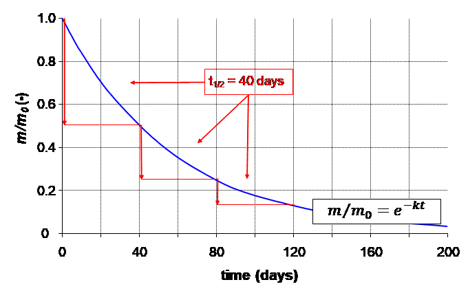
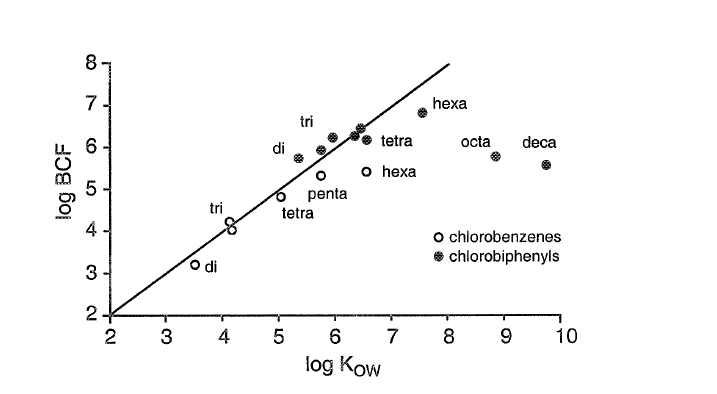
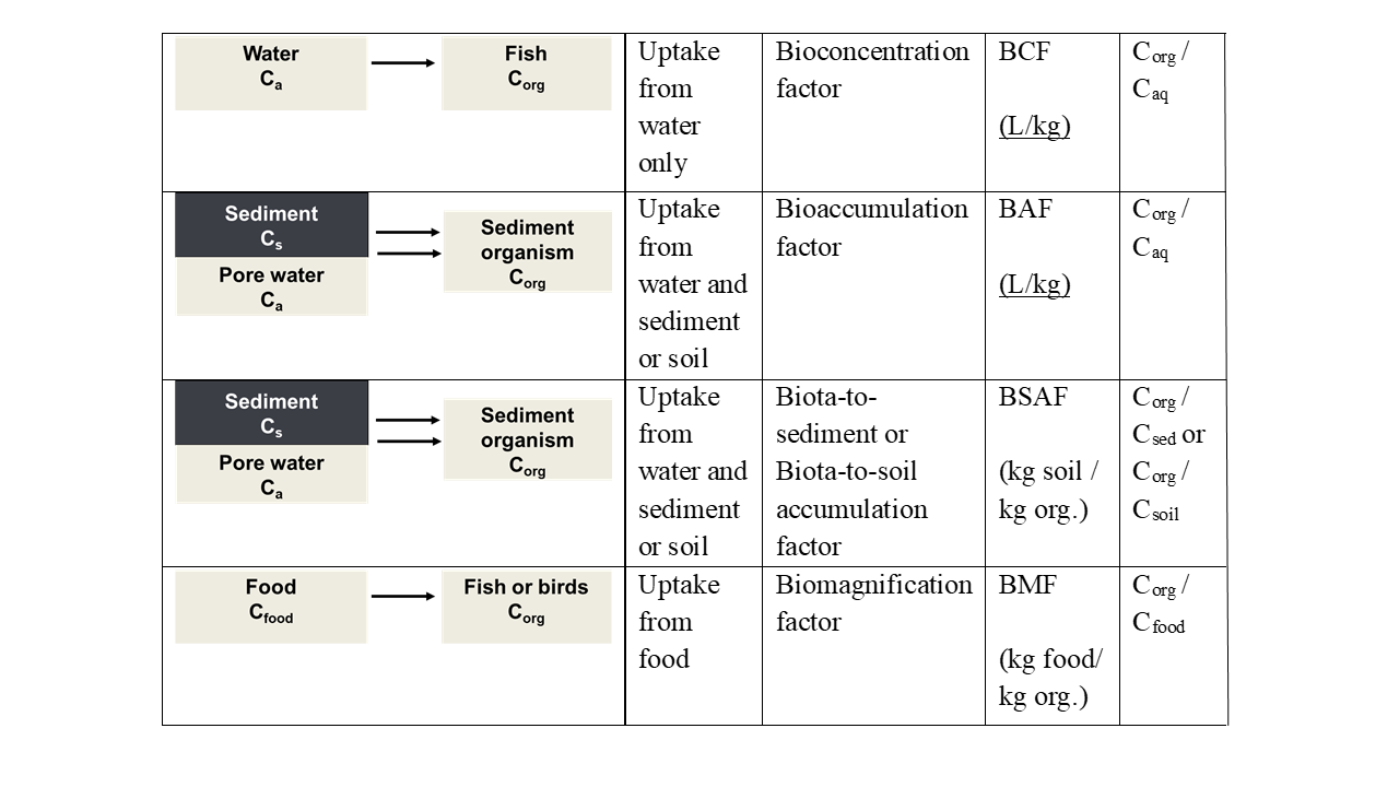
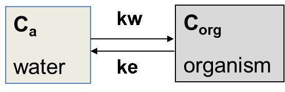
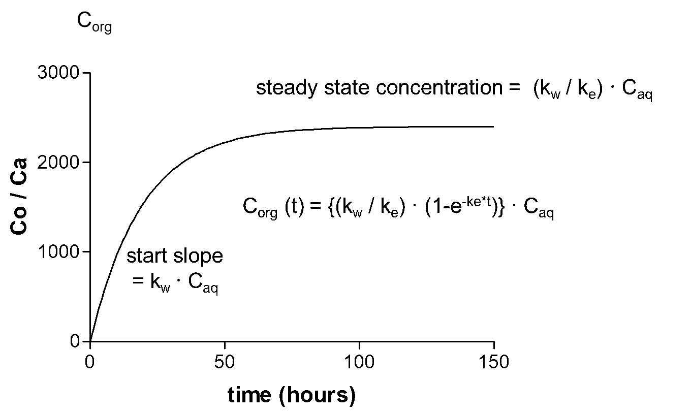
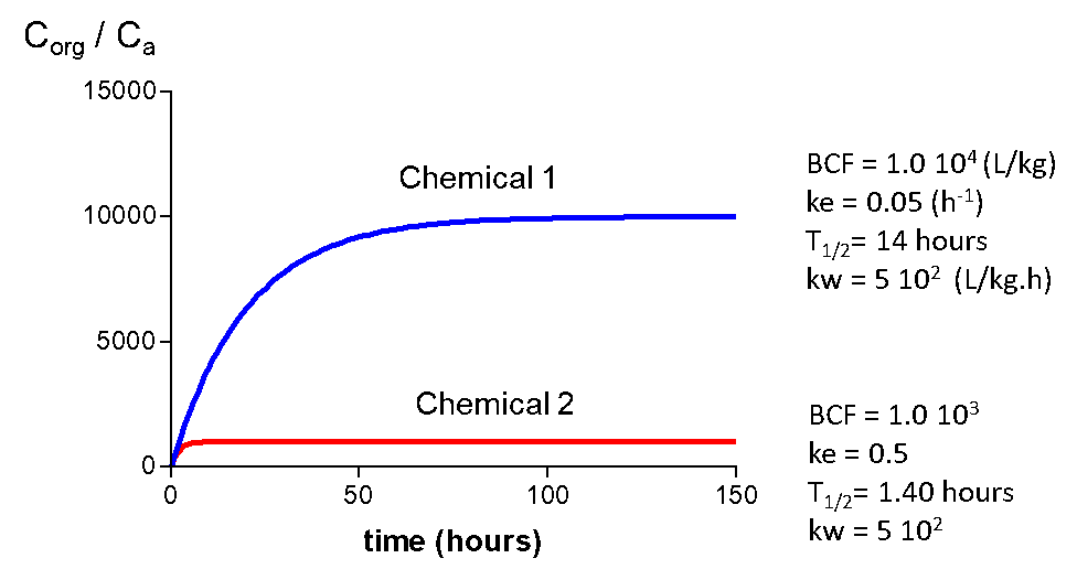
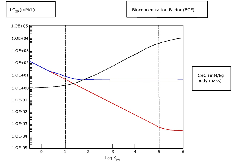
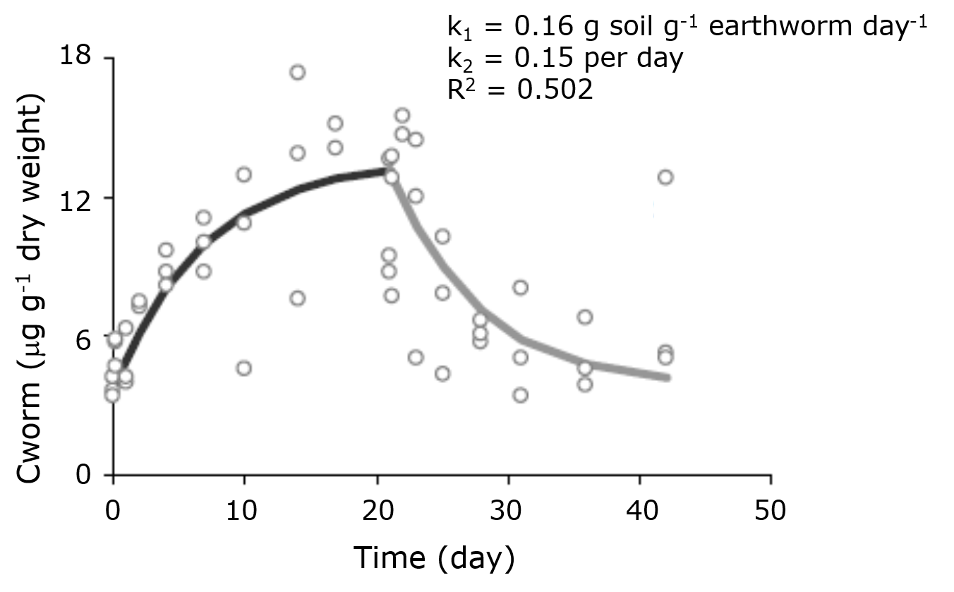
Corg/Caq becomes constant. This is the steady state situation. The constant Corg/Caq at steady state is called the bioconcentration factor BCF. Mathematically, the BCF can also be calculated from kw/ke. This follows directly from equation 4: after long exposure time (t),
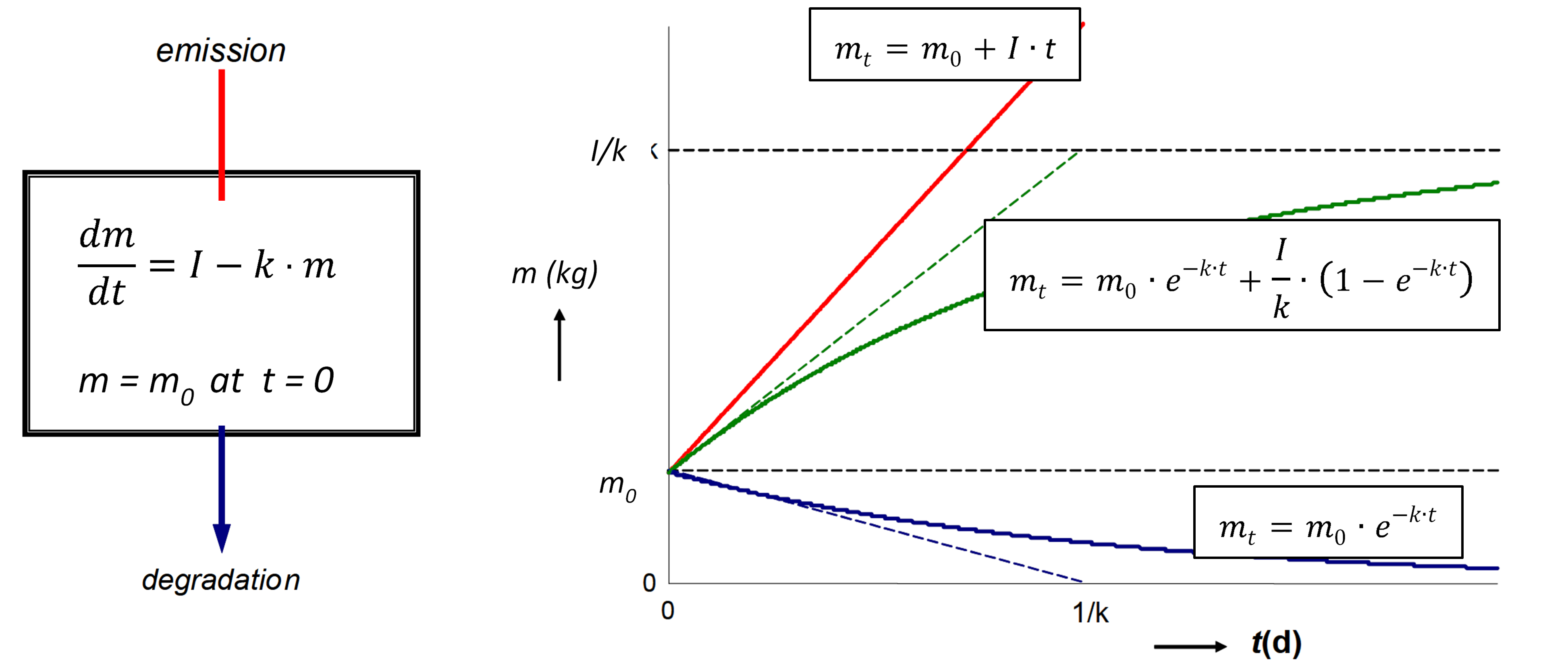
 \( e^{k_e t}\) becomes 0 leading to


\(C_{org} (t)= { k_w \over k_e } C_{aq} \)


\({C_{org} \over C_{aq}} (at\quad steady\quad state) = BCF = {k_w \over k_e} \)                                                           (7)


Elimination

Elimination is often measured following an uptake experiment. After the organism has reached a certain concentration, fish are transferred to a clean environment and concentration in the organism will decrease in time. Because this is also a first order kinetic process, the elimination rate will depend on the concentration in the organism (Corg) and the elimination rate constant (ke) (see equation 8). Concentration will decrease exponentially in time (equation 9) as shown in Figure 3A. Concentrations are often transformed to the natural logarithmic values (ln Corg) because this results in a linear relationship with slope -ke.(equation 10 and figure 3B).


\({dC_{org} \over dt}=- k_e C_{org}\)                                                                                 (8)


\(C_{org} (t)=C_{org} (t=0) e^{-k_e t}\)                                                                (9)


\(ln⁡ C_{org} (t) = ln⁡ C_{org} (t=0) - k_e t\)                                                      (10)


where Corg(t=0) is the concentration in the organism when the elimination phase starts.

The half-life (T1/2 or DT50) is the time needed to eliminate half the amount of chemical from the compartment. The relationship between ke and T1/2 is: T1/2 = (In 2) / ke. The half-life increases when ke decreases.

Figure 3. Elimination of a chemical from fish to water: one compartment model. Left: concentrations given on a normal scale. Right: concentration expressed as the natural logarithm to enable linear regression against time to yield the rate constant as the slope.


Multicompartment models

Very often, organisms cannot be considered as one compartment, but as two or even more compartments (Figure 4A). Deviations from the one-compartment system usually are seen when elimination does not follow an exponential pattern as expected: no linear relationship is obtained after logarithmic transformation. Figure 4B shows the typical trend of the elimination in a two-compartment system. The decrease in concentration (on a logarithmic scale) shows two phases: phase I with a relatively fast decrease and phase II with a relatively slow decrease. According to the linear compartment theory, elimination may be described as the sum of two (or more) exponential terms, like:


\(C_{org} (t) = C_{org} (t=0) F(I) e^{-k_e (I)*t}+F(II)e^{-k_e (II)*t}\)                               (11)


where

ke(I) and ke(II) represent elimination rate constants for compartment I and II,

F(I) and F(II) are the size of the compartments (as fractions)


Typical examples of two compartment systems are:

  • Blood (I) and liver (II)
  • Liver tissue (I) and fat tissue (II)

Elimination from fat tissue is often slower than from, for example, the liver. The liver is a well perfused organ while the exchange between lipid tissue and blood is much less. That explains the faster elimination from the liver.

Figure 4. Elimination of chemical from fish to water (top) in a two-compartment model (bottom).


Examples of uptake curves for different chemicals and organisms

Figure 5 gives uptake curves for two different chemicals and the corresponding kinetic parameters. Chemical 2 has a BCF of 1000, chemical 1 a BCF of 10,000. Uptake rates (kw) are the same, which is often the case for organic chemicals. Half-lives (time to reach 50 % of the steady state level) are 14 and 140 hours. This makes sense because it will take a longer time to reach steady state for a chemical with a higher BCF. Elimination rate constants also differ a factor of 10.

In figure 6, uptake curves are presented for one chemical, but in two organisms of different size/weight. Organism 1 is much smaller than organism 2 and reaches steady state much earlier. T1/2 values for the chemical in organisms 1 and 2 are 14 and 140 hours, respectively. The small size explains this fast equilibration. Rates of uptake depend on the surface-to-volume ratio (S/V) of an organism, which is much higher for a small organism. Therefore, kinetics in small organisms is faster resulting in shorter equilibration times. The effect of size on kinetics is discussed in more detail in Hendriks et al. (2001) and in the Section on Allometric Relationships.

Figure 5. Uptake curves for two chemicals, having different properties, in the same organism.


Figure 6. Uptake curves for the same chemical in two organisms having different sizes; organism 2 is much bigger than organism 1.


Bioaccumulation involving biotransformation and different routes of uptake

In equation 2, elimination only includes gill elimination. If other processes such as biotransformation and growth are considered, the equation can be extended to include these additional processes (see equation 12).


\({dC_{org} \over dt} = k_w C_a-(k_e+ k_m+ k_r ) C_{org} \)                                                      (12)


For organisms living in soil or sediment, different routes of uptake may be of importance: dermal (across the skin), or oral (by ingestion of food and/or soil or sediment particles). Mathematically, the uptake in an organism in sediment can be described as in equation 13.


\(C_{org} (t) = {( k_w C_{aq} + k_s C_s) \over k_e} (1- e^{-k_e t}) \)                                                            (13)


Corg       concentration in organisms (mg/kg)

Caq       concentration in aqueous phase (mg/L)

Cs        concentration soil or sediment (mg/kg)

kw        uptake rate constant from water (L/kg/day)

ks         uptake rate constant from soil or sediment (kgsoil/kgorganism/day)

ke         elimination rate constant (1/day)

t           time (day)

(dimensions used are: amount of chemical: mg; volume of water: L; weight of organism: kg; time: day)


In this equation, kw and ks are the uptake rate constants from water and sediment, ke is the elimination rate constant and Caq and Cs are the concentrations in water and sediment or soil. For soil organisms, such as earthworms, oral uptake appears to become more important with increasing hydrophobicity of the chemical (Jager et al., 2003). This is because the concentration in soil (Cs) will become higher than the porewater concentration Ca for the more hydrophobic chemicals (see section on Sorption).


References

Clewell, H.J., 3rd (1995). The application of physiologically based pharmacokinetic modeling in human health risk assessment of hazardous substances. Toxicology Letters 79, 207-217.

Hendriks, A.J., van der Linde, A., Cornelissen, G., Sijm, D. (2001). The power of size. 1. Rate constants and equilibrium ratios for accumulation of organic substances related to octanol-water partition ratio and species weight. Environmental Toxicology and Chemistry 20, 1399-1420.

Jager, T., Fleuren, R., Hogendoorn, E.A., De Korte, G. (2003). Elucidating the routes of exposure for organic chemicals in the earthworm, Eisenia andrei (Oligochaeta). Environmental Science and Technology 37, 3399-3404.

Nichols, J.W., Fitzsimmons, P.N., Whiteman, F.W. (2004). A physiologically based toxicokinetic model for dietary uptake of hydrophobic organic compounds by fish - II. Simulation of chronic exposure scenarios. Toxicological Sciences 77, 219-229.

Van Leeuwen, C.J., Vermeire, T.G. (Eds.) (2007). Risk Assessment of Chemicals: An Introduction. Springer, Dordrecht, The Netherlands.


4.1.3. Tissue accumulation of metals

Author: Nico M. van Straalen

Reviewers: Philip S. Rainbow, Henk Schat


Learning objectives:

You should be able to

  • indicate four types of inorganic metal binding cellular constituents present in biological tissues and indicate which metals they bind.
  • describe how phytochelatin and metallothionein are induced by metals.
  • mention a number of organ-metal combinations that are critical to metal toxicity.


Key words: Metal binding proteins; phytochelatin; metallothionein;


Synopsis

The issue of metal speciation, which is crucially important to understand metal fate in the environment, is equally important for internal distribution in organisms and toxicity inside the cell. Many metals tend to accumulate in specific organs, for example the hepatopancreas of crustaceans, the chloragogen tissue of annelids, and the kidney of mammals. In addition, there is often a specific organ or tissue where dysfunction or toxicity is first observed, e.g., in the human body, the primary effects of chronic exposure to mercury are seen in the brain, for lead in bone marrow and for cadmium in the kidney. This module is aimed at increasing the insight into the different mechanisms by which metals accumulate in biological tissues.


Introduction

Metals will be present in biological tissues in a large variety of chemical forms: free metal ion, various inorganic species with widely varying solubility, such as chlorides or carbonates, plus all kind of metal species bound to low-molecular and high-molecular weight biotic ligands. The free metal ion is considered the most relevant species relating to toxicity.

To explain the affinities of metals with specific targets, a system has been proposed based on the physical properties of the ion; according to this system, metals are divided into “oxygen-seeking metals” (class A, e.g. lithium, beryllium, calcium and lanthanum), and “sulfur-seeking metals” (class B, e.g. silver, mercury and lead) (See section on Metals and metalloids). However, most of the metals of environmental relevance fall in an intermediate class, called “borderline” (chromium, cadmium, copper, zinc, etc.). This classification is to some extent predictive of the binding of metals to specific cellular targets, such as SH-groups in proteins, nitrogen in histidine or carbonates in bone tissue.

Not only do metals differ enormously in their physicochemical properties, also the organisms themselves differ widely in the way they deal with metals. The type of ligand to which a metal is bound, and how this ligand is transported or stored in the body, determines to a great extent where the metal will accumulate and cause toxicity. Sensitive targets or critical biochemical processes differ between species and this may also lead to differential toxicity.


Inorganic metal binding

Many tissues contain “mineral concretions”, that is, granules with a specific mineral composition that, due to the nature of the mineral, attract different metals. Especially the gut epithelium of invertebrates, and their digestive glands (hepatopancreas, midgut gland, chloragogen tissue) may be full of such concretions. Four classes of granules are distinguished (Figure 1):

  • Calcium-pyrophosphate granules with magnesium, manganese, often also zinc, cadmium, lead and iron
  • Sulfur granules with copper, sometimes also cadmium
  • Iron granules, containing exclusively iron
  • Calcium carbonate granules, containing mostly calcium


Figure 1. Schematic diagram of the gut epithelium of an invertebrate animal, showing four different types of granules and the metals they usually contain. Redrawn from Hopkin (1989) by Wilma IJzerman.


The type B granules are assumed to be lysosomal vesicles that have absorbed metal-loaded peptides such as metallothionein or phytochelatin, and have developed into inorganic granules by degrading almost all organic material; the high sulfur content derives from the cysteine residues in the peptides.

Tissues or cells that specialize in the synthesis of intracellular granules are also the places where metals tend to accumulate. Well-known are the “S cells” in the hepatopancreas of isopods. These cells (small cells, B-type cells sensu Hopkin 1989) contain very large amounts of copper. Most likely the large stores of copper in woodlice and other crustaceans relate to their use of hemocyanin, a copper-dependent protein, as an oxygen-transporting molecule. Similar tissues with high loadings of mineral concretions have been described for earthworms, snails, collembolans and insects.


Organic metal binding

The second class of metal-binding ligands is of organic nature. Many plants but also several animals synthesize a peptide called phytochelatin (PC). This is an oligomer derived from glutathione with the three amino acids, γ-glumatic acid, cysteine and glycine, arranged in the following way: (γ-glu-cys)n-gly, where n can vary from 2 to 11. The thiol groups of several cysteine residues are involved in metal binding.

The other main organic ligand for metals is metallothionein (MT). This is a low-molecular weight protein with hydrophilic properties and an unusually large number of cysteine residues. Several cysteines (usually nine or ten) can bind a number of metal ions (e.g. four or five) in one cluster. There are two such clusters in the vertebrate metallothionein. Metallothioneins occur throughout the tree of life, from bacteria to mammals, but the amino acid sequence, domain structure and metal affinities vary enormously and it is doubtful whether they represent a single evolutionary-homologous group.

In addition to these two specific classes of organic ligands, MT and PC, metals will also bind aspecifically to all kind of cellular constituents, such as cell wall components, albumen in the blood, etc. Often this represents the largest store of metals; such aspecific binding sites will constantly deliver free metal ions to the cellular pool and so are the most important cause of toxicity. Of course metals are also present in molecules with specific metal-dependent functions, such as iron in hemoglobin, copper in hemocyanin, zinc in carbonic anhydrase, etc.

The distinction between inorganic ligands and organic ones is not as strict as it may seem. After binding to metallothionein or phytochelatin metals may be transferred to a more permanent storage compartment, such as the intracellular granules mentioned above, or they may be excreted.


Regulation of metal binding

Free metal ions are strong inducers of stress response pathways. This can be due to the metal ion itself but more often the stress response is triggered by a metal-induced disturbance of the redox state, i.e. an induction of oxidative stress. The stress response often involves the synthesis of metal-binding ligands such as phytochelatin and metallothionein. Because this removes metal ions from the active pool it is also called metal scavenging.

The binding capacity of phytochelatin is enhanced by activation of the enzyme phytochelatin synthase (PC synthase). According to one model of its action, the C-terminus of the enzyme has a “metal sensor” consisting of a number of cysteines with free SH-groups. Any metal ions reacting with this nucleophile center (and cadmium is a strong reactant) will activate the enzyme which then catalyzes the reaction from (γ-glu-cys)n-gly to (γ-glu-cys)n+1-gly, thus increasing the binding capacity of cellular phytochelatin (Figure 2). This reaction of course relies on the presence of sufficient glutathione in the cell. In plants the PC-metal complex is transported into the central vacuole, where it can be stabilized through incorporation of acid-labile sulfur (S2). The PC moiety is degraded, resulting in the formation of inorganic metal-sulfide crystallites. Alternatively, complexes of metals with organic acids may be formed (e.g. citrates or oxalates). The fate of metal-loaded PC in animal cells is not known, but it might be absorbed in the lysosomal system to form B-type granules (see above).


Figure 2. Model for the regulation of phytochelatin synthase, an enzyme catalyzing the extension of phytochelatin and increasing the binding capacity for metals. From Cobbet (2000). Source: http://www.plantphysiol.org/content/123/3/825


The upregulation of metallothionein (MT) occurs in a quite different manner, since it depends on de novo synthesis of the apoprotein. It is a classic example of gene regulation contributing to protection of the cell. In a wide variety of animals, including vertebrates and invertebrates, metallothionein genes (Mt) are activated by a transcription factor called metal-responsive transcription factor 1 (MTF-1). MTF -1 binds to so-called metal-responsive elements (MREs) in the promoter of Mt. MREs are short motives with a characteristic base-pair sequence that form the core of a transcription factor binding site in the DNA. Under normal physiological conditions MTF-1 is inactive and unable to induce Mt. However, it may be activated by Zn2+ ions, which are released, from unspecified ligands, by metals such as cadmium that can replace zinc (Figure 3).


Figure 3. Model for metallothionein induction by cadmium. Cadmium ions (Me) displace zinc ions from ligands (MP). Free zinc ions (Zn) then activate Metal Transcription Factor 1 (MTF-1) in the nucleus to bind to transcription factor binding sites containing Metal-Responsive Elements (MRE). This induces expression of Mt and other genes. These genes may also be induced by oxidative stress, acting upon antioxidant-responsive elements (ARE) and Enhancer Box (E box). Oxidative stress may come from external oxidizing agents or from the metal itself. Finally, zinc ions may also directly activate antioxidant enzymes. Adapted from Haq et al. (2003) by Wilma IJzerman.


It must be emphasized that the model discussed above is inspired by work on vertebrates. Arthropods (Drosophila, Orchesella, Daphnia) could have a similar mechanism since they also have an MTF-1 homolog that activates Mt, however, the situation for other invertebrates such as annelids and gastropods is unclear; their Mt genes seem to lack MREs, despite being inducible by cadmium. In addition, the variability of metallothioneins in invertebrates is extremely large and not all metal-binding proteins may be orthologs of the vertebrate metallothionein. In snails, a cadmium-binding, cadmium-induced MT functions alongside a copper-binding MT while the two MTs have different tissue distributions and are also regulated quite differently.

While both phytochelatin and metallothionein will sequester essential as well as non-essential metals (e.g. Cd) and so contribute to detoxification, the widespread presence of these systems throughout the tree of life suggests that they did not evolve primarily to deal with anthropogenic metal pollution. The very strong inducibility of these systems by non-essential elements like cadmium may be considered a side-effect of a different primary function, for example regulation of the cellular redox state or binding of essential metals.


Target organs

Any tissue-specific accumulation of metals can be explained by turnover of metal-binding ligands. For example, accumulation of cadmium in mammalian kidney is due to the fact that metallothionein loaded with cadmium cannot be excreted. High concentrations of metals in the hind segments of earthworms are due to the presence of “residual bodies” which are fully packed with intracellular granules. Accumulation of cadmium in the human prostrate is due to the high concentration of zinc citrate in this organ, which serves to protect contractile proteins in sperm tails from oxidation; cadmium assumedly enters the prostrate through zinc transporters.

It is often stated that essential metals are subject to regulatory mechanisms, which would imply that their body burden, over a large range of external exposures, is constant. However, not all “essential” metals are regulated to the extent that the whole-body concentration is kept constant. Many invertebrates have body compartments associated with the gut (midgut gland, hepatopancreas, Malpighian tubules) in which metals, often in the form of mineral concretions, are inactivated and stored permanently or exchanged very slowly with the active pool. Since these compartments are outside the reach of regulatory mechanisms but usually not separated in whole-body metal analysis, the body burden as a whole is not constant. Some invertebrates even carry a “backpack” of metals accumulating over life. This holds, e.g., for zinc in barnacles, copper in isopods and zinc in earthworms.

Accumulation of metals in target organs may lead to toxicity when the critical binding or excretion capacity is exhausted and metal ions start binding aspecifically to cellular constituents. The organ in which this happens is often called the target organ. The total metal concentration at which toxicity starts to become apparent is called the critical body concentration (CBC) or critical tissue concentration. For example, the critical concentration for cadmium in kidney, above which renal damage is observed to occur, is estimated to be 50 μg/g. A list of critical organs for metals in the human body is given in Table 1.

The concept of CBC assumes that the complete metal load in an organ is in equilibrium with the active fraction causing toxicity and that there is no permanent storage pool. In the case of storage detoxification the body burden at which toxicity appears will depend on the accumulation history.


Table 1. Critical organs for chronic toxicity of metals in the human body

Metal or metalloid

Critical organ

Symptoms

Al

Brain

Alzheimer’s disease

As

Lung, liver, heart gut

Multisystem energy disturbance

Cd

Kidney, liver

Kidney damage

Cr

Skin, lung, gut

Respiratory system damage

Cu

Liver

Liver damage

Hg

Brain, liver

Mental illness

Ni

Skin, kidney

Allergic reaction, kidney damage

Pb

Bone marrow, blood, brain

Anemia, mental retardation


References

Cobbett, C., Goldsbrough, P. (2002). Phytochelatins and metallothioneins: roles in heavy metal detoxification and homeostasis. Annual Review of Plant Biology 53, 159-182.

Dallinger, R., Berger, B., Hunziker, P., Kägi, J.H.R. (1997). Metallothionein in snail Cd and Cu metabolism. Nature 388, 237-238.

Dallinger, R., Höckner, M. (2013). Evolutionary concepts in ecotoxicology: tracing the genetic background of differential cadmium sensitivities in invertebrate lineages. Ecotoxicology 22, 767-778.

Haq, F., Mahoney, M., Koropatnick, J. (2003) Signaling events for metallothionein induction. Mutation Research 533, 211-226.

Hopkin, S.P. (1989) Ecophysiology of Metals in Terrestrial Invertebrates. London, Elsevier Applied Science.

Nieboer, E., Richardson, D.H.S. (1980) The replacement of the nondescript term "heavy metals" by a biologically and chemically significant classification of metal ions. Environmental Pollution Series B 1, 3-26.

Rainbow, P.S. (2002) Trace metal concentrations in aquatic invertebrates: why and so what? Environmental Pollution 120, 497-507.

4.1.4. Xenobiotic defence and metabolism

Author: Nico M. van Straalen

Reviewers: Timo Hamers, Cristina Fossi


Learning objectives:

You should be able to:

  • recapitulate the phase I, II and III mechanisms for xenobiotic metabolism, and the most important molecular systems involved.
  • describe the fate and the chemical changes of an organic compound that is metabolized by the human body, from absorption to excretion.
  • explain the principle of metabolic activation and why some compounds can become very reactive upon xenobiotic metabolism.
  • develop a hypothesis on the ecological effects of xenobiotic compounds that require metabolic activation.


Keywords: biotransformation; phase 1; phase II; phase III; excretion; metabolic activation; cytochrome P450


Synopsis

All organisms are equipped with metabolic defence mechanisms to deal with foreign compounds. The reactions involved, jointly called biotransformation,  can be divided into three phases, and usually aim to increase water solubility and excretion. The first step (phase I) is catalyzed by cytochrome P450, which is followed by a variety of conjugation reactions (phase II) and excretion (phase III). The enzymes and transporters involved are often highly inducible, i.e. the amount of protein is greatly enhanced by the xenobiotic compounds themselves. The induction involves binding of the compound to cytoplasmic receptor proteins, such as the arylhydrocarbon receptor (AhR), or the constitutive androstane receptor (CAR). In some cases the intermediate metabolites, produced in phase I are extremely reactive and a main cause of toxicity, a well-known example being the metabolic activation of polycyclic aromatic hydrocarbons such as benzo(a)pyrene, which readily forms DNA adducts and causes cancer. In addition, some compounds greatly induce metabolizing enzymes but are hardly degraded by them and cause chronic cellular stress. The various biotransformation reactions are a crucial aspect of both toxicokinetics and toxicodynamics of xenobiotics.


Introduction

The term “xenobiotic” (“foreign to biology”) is generally used to indicate a chemical compound that does not normally have a metabolic function. We will use the term extensively in this module, despite the fact that it is somewhat problematic (e.g., can a compound be considered “foreign” if it circulates in the body, is metabolized or degraded in the body?, and: what is “foreign” for one species is not necessarily “foreign” for another species).

The body has an extensive defence system to deal with xenobiotic compounds, loosely designated as biotransformation. The ultimate result of this system is excretion the compound in some form or another. However, many xenobiotics are quite lipophilic, tend to accumulate and are not easily excreted due to low water solubility. Molecular modifications are usually required before such compounds can be removed from the body, as the main circulatory and excretory systems (blood, urine) are water-based. By introducing hydrophilic groups in the molecule (-OH, =O, -COOH) and by conjugating it to an endogenous compound with good water-solubility, excretion is usually accomplished. However, as we will see below, intermediate metabolites may have enhanced reactivity and it often happens that a compound becomes more toxic while being metabolized. In the case of pesticides, deliberate use is made of such responses, to increase the toxicity of an insecticide once it is in the target organism.

The study of xenobiotic metabolism is a classical subject not only in toxicology but also in pharmacology. The mode of action of a drug often depends critically on the rate and mode of metabolism. Also, many drugs show toxic side-effects as a consequence of metabolism. Finally, xenobiotic metabolism is also studied extensively in entomology, as both toxicity and resistance of pesticides are often mediated by metabolism.

The most problematic xenobiotics are those with a high octanol-water partition coefficient (Kow) that are strongly lipophilic and very hydrophobic. They tend to accumulate, in proportion to their Log Kow, in tissues with a high lipid content such as the subcutis of vertebrates, and may cause tissue damage due to disturbance of membrane functions. This mode of action is called “minimum toxicity”. Well-known are low-molecular weight aliphatic petroleum compounds and chlorinated alkanes such as chloroform. These compounds cause their primary damage to cell membranes; especially neurons are sensitive to this effect, hence minimum toxicity is also called narcotic toxicity. Lipophilic chemicals with high Log Kow do not reach concentrations high enough to cause minimum toxicity because they induce biotransformation at lower concentrations. The toxicity is then usually due to a reactive metabolite.

Xenobiotic metabolism involves three subsequent phases (Figure 1):

  1. Activation (usually oxidation) of the compound by an enzyme known as cytochrome P450, which acts in cooperation with NADPH cytochrome P450 reductase and other factors.
  2. Conjugation of the activated product of phase I to an endogenous compound. A host of different enzymes is available for this task, depending on the compound, the tissue and the species. There are also (slightly polar) compounds that enter phase II directly, without being activated in phase I.
  3. Excretion of the compound into circulation, urine, or other media, usually by means of membrane-spanning transporters belonging to the class of ATP-binding cassette (ABC) transporters, including the infamous multidrug resistance proteins. Hydrophilic compounds may pass on directly to phase III, without being activated or conjugated.


Figure 1. The various phases of xenobiotic metabolism. Redrawn by Wilma Ijzerman.


Phase I reactions

Cytochrome P450 is a membrane-bound enzyme, associated with the smooth endoplasmic reticulum. It carries a porphyrin ring containing an Fe atom, which is the active center of the molecule. The designation P450 is derived from the fact that it shows an absorption maximum at 450 nm when inhibited by carbon monoxide, a now outdated method to demonstrate its presence. Other (outdated) namings are MFO (mixed function oxygenase) and drug metabolizing enzyme complex. Cytochrome P450 is encoded by a gene called CYP, of which there are many paralogs in the genome, all slightly differing from each other in terms of inducibility and substrate specificity. Three classes of CYP genes are involved with biotransformation, designated CYP1, CYP2 and CYP3 in vertebrates. Each class has several isoforms; the human genome has 57 different CYP genes in total. The CYP complement of invertebrates and plants often involves even more genes; many evolutionary lineages have their own set, arising from extensive gene duplications within that lineage. In humans, the genetic complement of a person’s CYP genes is highly relevant as to its drug metabolizing profile (see the section on Genetic variation in toxicant metabolism).

Cytochrome P450 operates in conjunction with an enzyme called NADPH cytochrome P450 reductase, which consists of two flavoproteins, one containing Flavin adenine dinucleotide (FAD), the other flavin mononucleotide (FMN). The reduced Fe2+ atom in cytochrome P450 binds molecular oxygen, and is oxidized to Fe3+ while splitting O2; one O atom is introduced in the substrate, the other reacts with hydrogen to form water. Then the enzyme is reduced by accepting an electron from cytochrome P450 reductase. The overall reaction can be written as:

         RH + O2 + NADPH + H+ → ROH + H2O + NADP+

where R is an arbitrary substrate.


Cytochrome P450 is expressed to a great extent in hepatocytes (liver cells), the liver being the main organ for xenobiotic metabolism in vertebrates (Figure 2), but it is also present in epithelia of the lung and the intestine. In insects the activity is particularly high in the Malpighian tubules in addition to the gut and the fat body. In mollusks and crustaceans the main metabolic organ is the hepatopancreas.


Phase II reactions

After activation by cytochrome P450 the oxidized substrate is ready to be conjugated to an endogenous compound, e.g. a sulphate, glucose, glucuronic acid or glutathione group. These reactions are conducted by a variety of different enzymes, of which some reside in the sER like P450, while others are located in the cytoplasm of the cell (Figure 2). Most of them transfer a hydrophilic group, available from intermediate metabolism, to the substrate, hence the enzymes are called transferases. Usually the compound becomes more polar in phase II, however, not all phase II reactions increase water solubility; for example, methylation (by methyl transferase) decreases reactivity but increases apolarity. Other phase II reactions are conjugation with glutathione, conducted by glutathione-S-transferase (GST) and with glucuronic acid, conducted by UDP-glucuronyl transferase. In invertebrates other conjugations may dominate, e.g. in arthropods and plants, conjugation with malonyl glucose is a common reaction, which is not seen in vertebrates.

Conjugation with glutathione in the human body is often followed by splitting off glutamic acid and glycine, leaving only the cysteine residue on the substrate. Cysteine is subsequently acetylated, thus forming a so-called mercapturic acid. This is the most common type of metabolite for many xenobiotics excreted in urine by humans.

Like cytochrome P450, the phase II enzymes consist in various isoforms, encoded by different paralogs in the genome. Especially the GST family is quite extensive and polymorphisms in these genes contribute significantly to the personal metabolic profile (see the section on Genetic variation in toxicant metabolism).


Figure 2. Schematic view of xenobiotic metabolism (phase I and phase II) in human liver. P450 = cytochrome P450, FP = flavoprotein, RED = cytochrome P450 reductase, EH = epoxide hydrolase, UDP-GT = uridyldiphospho-glucuronyl transferase, GSH-T = glutathione-S-transferase, ST = sulphotransferase. Reproduced from Vermeulen & Van den Broek (1984) by Wilma Ijzerman.


Phase III reactions

In the human body, there are two main pathways for excretion, one from the liver into the bile (and further into the gut and the faeces), the other through the kidney and urine. These two pathways are used by different classes of xenobiotics: very hydrophobic compounds such as high-molecular weight polycyclic aromatic hydrocarbons are still not readily soluble in water even after metabolism but can be emulsified by bile salt and excreted in this way. It sometimes happens that such compounds, once arriving in the gut, are assimilated again, transported to the liver by the portal vein and metabolized again. This is called “entero-hepatic circulation”. Lower molecular weight compounds and hydrophilic compounds are excreted through urine. Volatile compounds can leave the body through the skin and exhaled air.

Excretion of activated and conjugated compounds from tissues out of the cell usually requires active transport, which is mediated by ABC (ATP binding cassette) transporters, a very large and diverse family of membrane proteins which have in common a binding cassette for ATP. Different subgroups of ATP transporters transport different types of chemicals, e.g. positively charged hydrophobic molecules, neutral molecules and water-soluble anionic compounds. One well-known group consists of multidrug resistance proteins or P-glycoproteins. These transporters export drugs aiming to attack tumor cells. Because their activity is highly inducible, these proteins can enhance excretion enormously, making the cell effectively resistant and thus case major problems for cancer treatment.


Induction

All enzymes of xenobiotic metabolism are highly inducible: their activity is normally on a low level but is greatly enhanced in the presence of xenobiotics. This is achieved through a classic case of transcriptional regulation upon CYP and other genes, leading to de novo synthesis of protein. In addition, extensive proliferation of the endoplasmic reticulum may occur, and in extreme cases even swelling of the liver (hepatomegaly).

The best investigated pathway for transcriptional activation of CYP genes is due to the arylhydrocarbon receptor (AhR). Under normal conditions, this peptide is stabilized in the cytoplasm by heat-shock proteins, however, when a xenobiotic compound binds to AhR, it is activated and can join with another protein called Ah receptor nuclear translocator (ARNT) to translocate to the nucleus and bind to DNA elements present in the promotor of CYP and other genes. It thus acts as a transcriptional activator or transcription factor on these genes (Figure 3). The DNA motifs to which AhR binds are called xenobiotic responsive elements (XRE) or dioxin-responsive elements (DRE). The compounds acting in this manner are called 3-MC-type inducers, after the (highly carcinogenic) model compound 3-methylcholanthrene. The inducing capacity of a compound is related to its binding affinity to the AhR, which in itself is determined by the spatial structure of the molecule. The lock-and key fitting between AhR and xenobiotics explains why induction of biotransformation by xenobiotics shows a very strong stereospecificity. For example, among the chlorinated biphenyls and chlorinated dibenzodioxins, some compounds are extremely strong inducers of CYP1 genes, while others, even with the same number of chlorine atoms, are no inducers at all. The precise position of the chlorine atoms determines the molecular “fit” in the Ah receptor (see Section on Receptor interaction).

In addition to 3MC-type of induction there are other modes in which biotransformation enzymes are induced, but these are less well-known. A common class is PB-type induction (named after another model compound, phenobarbital). PB-type induction is not AhR-dependent, but acts through activation of another nuclear receptor, called constitutive androstane receptor (CAR). This receptor activates CYP2 genes and some CYP3 genes.

The high inducibility of biotransformation can be exploited in a reverse manner: if biotransformation is seen to be highly upregulated in a species living in the environment, this indicates that that species is being exposed to xenobiotic compounds. Assays addressing cytochrome P450 activity can therefore be exploited in bioindication and biomonitoring systems. The EROD (ethoxyresorufin-O-deethylase) assay is often used for this purpose, although it is not 100% specific to the isoform of P450. Another approach is to address CYP expression directly, e.g. through reverse transcription-quantitative PCR, a method to quantify the amount of CYP mRNA.


Figure 3. Scheme illustrating how AhR-reactive compounds induce biotransformation activity. 1 xenobiotic compounds enter the cell through diffusion, 2 compound binds to AhR, releasing it from Hsp90, 3 AhR complex is activated by ARNT, 4 translocation to nucleus, 5 binding to XRE, 6 enhanced transcription, 7 translocation of mRNA to cytoplasm and translation, 8 incorporation of P450 enzyme in sER and biotransformation of compounds. AhR = arylhydrocarbon receptor, Hsp90 = heat shock protein 90, ARNT = aryl hydrocarbon nuclear translocator, XRE = xenobiotic responsive element, CYP1 = gene encoding cytochrome P450 1, sER = smooth endoplasmic reticulum. Drawn by Wilma Ijzerman.


Secondary effects of biotransformation

Although the main aim of xenobiotic metabolism is to detoxify and excrete foreign compounds, some pathways of biotransformation actually enhance toxicity. This is mostly due to the first step, activation by cytochrome P450. The activation may lead to intermediate metabolites which are highly reactive and the actual cause of toxicity. The best investigated examples are due to bioactivation of polycyclic aromatic hydrocarbons (PAHs), a group of chemicals present in diesel, soot, cigarette smoke and charred food products. Many of these compounds, e.g. benzo(a)pyrene, benz(a)anthracene and 3-methylcholanthrene, are not reactive or toxic as such but are activated by cytochrome P450 to extremely reactive molecules. Benzo(a)pyrene, for instance, is activated to a diol-epoxide, which readily binds to DNA, especially to the free amino-group of guanine (Figure 4). The complex is called a DNA adduct, the double helix is locally disrupted and this results in a mutation. If this happens in an oncogene, a tumor may develop (see the Section on Carcinogenesis and genotoxicity).

Not all PAHs are carcinogenic. Their activity critically depends on the spatial structure of the molecule, which again determines its “fit” in the Ah receptor. PAHs with a “notch” (often called bay-region) in the molecule tend to be stronger carcinogens than compounds with a symmetric (round or linear) molecular structure.


Figure 4. Metabolism of benzo(a)pyrene (B[a]P) to a mutagenic and carcinogenic metabolite, BaP-diol epoxide. Cytochrome P450 activity (CYP1A1 and CYP1B1) introduces an epoxide on the 7,8 position of the molecule, which is then hydrolyzed by epoxide hydrolase to a dihydrodiol (two OH groups next to each other, which can be in trans position, pointing in different directions relative to the plane of the molecule, or in cis, pointing in the same direction). The trans metabolite is preferably formed. Subsequently another epoxide is introduced on the 9,10 position. The diolepoxide is highly reactive, and may bind proteins and to guanine in DNA, causing a DNA adduct. Modified from Bui et al. (2009) by Steven Droge.


Another mechanism for biotransformation-induced toxicity is due to some very recalcitrant organochlorine compounds such as polychlorinated dibenzodioxins (PCDDs, or dioxins for short) and polychlorinated biphenyls (PCBs). Some of these compounds are very potent inducers of biotransformation, but they are hardly degraded themselves. The consequence is that the highly upregulated cytochrome P450 activity continues to generate a large amount of reactive oxygen (ROS), causing oxidative stress and damage to cellular constituents. It is assumed that the chronic toxicity of 2,3,7,8-tetrachlorodibenzo(para)dioxin (TCDD), one of the most toxic compounds emitted by human activity, is due to its high capacity to induce prolonged oxidative stress. On the molecular level, there is a close link between oxidative stress and biotransformation activity. Many toxicants that primarily induce oxidative stress (e.g. cadmium) also upregulate CYP enzymes. Two defence mechanisms, oxidative stress defence and biotransformation are part of the same integrated stress defence system of the cell.


References

Bui, P.H., Hsu, E.L., Hankinson, O. (2009), Fatty acid hydroperoxides support cytochrome P450 2S1-mediated bioactivation of benzo[a]pyrene-7-8-dihydrodiol. Molecular Pharmacology 76, 1044-1052.

Stroomberg, G.J., Zappey, H., Steen, R.J.C.A., Van Gestel, C.A.M., Ariese, F., Velthorst, N.H., Van Straalen, N.M. (2004). PAH biotransformation in terrestrial invertebrates – a new phase II metabolite in isopods and springtails. Comparative Biochemistry and Physiology Part C 138, 129-137.

Timbrell, J.A. (1982). Principles of Biochemical Toxicology. Taylor & Francis Ltd, London.

Van Straalen, N.M., Roelofs, D. (2012). An Introduction to Ecological Genomics, 2nd Ed. Oxford University Press, Oxford.

Vermeulen, N.P.E., Van den Broek, J.M. (1984). Opname en verwerking van chemicaliën in de mens. Chemisch Magazine. Maart: 167-171.


4.1.5. Allometric relationships

Author: A. Jan Hendriks

Reviewers: Nico van den Brink, Nico van Straalen


Learning objectives:

You should be able to

  • explain why allometrics is important in risk assessment across chemicals and species
  • summarize how biological characteristics such as consumption, lifespan and abundance scale size
  • describe how toxicological quantities such as uptake rates and lethal concentrations scale to size


Keywords: body size, biological properties, scaling, cross-species extrapolation, size-related uptake kinetics


Introduction

Globally more than 100,000,000 chemicals have been registered. In the European Union more than 100,000 compounds are awaiting risk assessment to protect ecosystem and human health, while 1,500,000 contaminated sites potentially require clean-up. Likewise, 8,000,000 species, of which 10,000 are endangered, need protection worldwide, with one lost per hour (Hendriks, 2013). Because of financial, practical and ethical (animal welfare) constraints, empirical studies alone cannot cover so many substances and species, let alone their combinations. Consequently, the traditional approach of ecotoxicological testing is gradually supplemented or replaced by modelling approaches. Environmental chemists and toxicologists for long have developed relationships allowing extrapolation across chemicals. Nowadays, so-called Quantitative Structure Activity Relationships (QSARs) provide accumulation and toxicity estimates for compounds based on their physical-chemical properties. For instance bioaccumulation factors and median lethal concentrations have been related to molecular size and octanol-water partitioning, characteristic properties of a chemical that are usually available from its industrial production process.

In analogy with the QSAR approach in environmental chemistry, the question may be asked whether it is possible to predict toxicological, physiological and ecological characteristics of species from biological traits, especially traits that are easily measured, such as body size. This approach has gone under the name “Quantitative Species Sensitivity Relationships” (QSSR) (Notenboom, 1995).

Among the various traits available, body-size is of particular interest. It is easily measured and a large part of the variability between organisms can be explained from body size, with r2 > 0.5. Not surprisingly, body size also plays an important role in toxicology and pharmacology. For instance, toxic endpoints, such as LC50s, are often expressed per kg body weight. Recommended daily intake values assume a “standard” body weight, often 60 kg. Yet, adult humans can differ in body weight by a factor of 3 and the difference between mouse and human is even larger. Here it will be explored how body-size relationships, which have been studied in comparative biology for a long time, affect the extrapolation in toxicology and can be used to extrapolate between species.


Fundamentals of scaling in biology

Do you expect a 104 kg elephant to eat 104 times more than a 1 kg rabbit per day? Or less, or more? On being asked, most people intuitively come up with the right answer. Indeed, daily consumption by the proboscid is less than 104 times that of the rodent. Consequently, the amount of food or water used per kilogram of body weight of the elephant is less than that of the rabbit. Yet, how much less exactly? And why should sustaining 1 kg of rabbit tissue require more energy than 1 kg of elephant flesh in the first place?

A century of research (Peters, 1983) has demonstrated that many biological characteristics Y scale to size X according to a power function:

Y = a Xb

where the independent variable X represents body mass, and the dependent variable Y can virtually be any characteristic of interest ranging, e.g., from gill area of fish to density of insects in a community.

Plotted in a graph, the equation produces a curved line, increasing super-linearly if b > 1 and sub-linearly if b < 1. If b=1, Y and X are directly proportional and the relationship is called isometric. As curved lines are difficult to interpret, the equation is often simplified by taking the logarithm of the left and right parts. The formula then becomes:

log Y = log a + b log X

When log Y is plotted against log X, a straight line results with slope b and intercept log a. If data are plotted in this way, the slope parameter b may be estimated by simple linear regression.

Across wide size ranges, slope b often turns out to be a multitude of ¼ or, occasionally, ⅓. Rates [kg∙d-1] of consumption, growth, reproduction, survival and what not, increase with mass to the power ¾ , while rate constants, sometimes called specific rates [kg∙kg-1∙d-1], decrease with mass to the power –¼. So, while the elephant is 104 kg heavier than the 1 kg rabbit, it eats only (104)¾ = 103 times more each day. Vice versa, 1 kg of proboscid apparently requires a consumption of (104) kg∙kg-1∙d-1, i.e., 10 times less. Variables with a time dimension [d] like lifespan or predator-prey oscillation periods scale inversely to rate constants and thus change with body mass to the power ¼. So, an elephant becomes (104)¼ = 10 times older than a rabbit. Abundance, i.e., the number of individuals per surface area [m-2] decreases with body mass to the power –¾. Areas, such as gill surface or home range, scale inversely to abundance, typically as body mass to the power ¾.

Now, why would sustaining 1 kg of elephant require 10 times less food than 1 kg of rabbit? Biologists, pharmacologists and toxicologists first attributed this difference to area-volume relationships. If objects of the same shape but different size are compared, the volume increases with length to the power 3 and the surface increases with length to the power 2. For a sphere with radius r, for example, area A and volume V increase as A ~ r2 and V ~ r3, so area scales to volume as A ~ r2 ~ (V)2 ~ V. So, larger animals have relatively smaller surfaces, as long as the shape of the organism remains the same. Since many biological processes, such as oxygen and food uptake or heat loss deal with surfaces, metabolism was, for long, thought to slow down like geometric structures, i.e., with multitudes of ⅓. Yet, empirical regressions, e.g. the “mouse-elephant curve” developed by Max Kleiber in the early 1930s show a universal slope of ¼ (Peters, 1983. This became known as the “Kleiber’s law”. While the data leave little doubt that this is the case, it is not at all clear why it should be ¼ and not ⅓. Several explanations for the ¼ slope have been proposed but the debate on the exact value as well as the underlying mechanism continues.


Application of scaling in toxicology

Since chemical substances are carried by flows of air and water, and inside the organism by sap and blood, toxicokinetics and toxicodynamics are also expected to scale to size. Indeed, data confirm that uptake and elimination rate constants decrease with size, with an exponent of about –¼ (Figure 1). Slopes vary around this value, the more so for regressions that cover small size ranges and physiologically different organisms. The intercept is determined by resistances in unstirred water layers and membranes through which the substances pass, as well as by delays in the flows by which they are carried. The resistances mainly depend on the affinity and molecular size of the chemicals, reflected by, e.g., the octanol-water partition coefficient Kow for organic chemicals or atomic mass for metals. The upper boundary of the intercept is set by the delays imposed by consumption and, subsequently, egestion and excretion. The lower end is determined by growth dilution. Both uptake and elimination scale to mass with the same exponent so that their ratio, reflecting the bioconcentration or biomagnification factor in equilibrium, is independent of body-size.


Figure 1. Regressions of elimination rate constants [kg∙kg-1∙d-1 = d-1] as a function of organism mass m [kg], ranging from algae to mammals, and organic chemicals' octanol-water partition ratio Kow and metal mass within the limits set by consumption and production (redrawn by author, based on Hendriks et al. 2001).


Scaling of rate constants for uptake and elimination, such as in Figure 1, implies that small organisms reach a given internal concentration faster than large ones. Vice versa, lethal concentrations in water or food needed to reach the same internal level after equal (short-term) exposure duration are lower in smaller compared to larger organisms. Thus, the apparent "sensitivity" of daphnids can, at least partially, be attributed to their small body-size. This emphasizes the need to understand simple scaling relationships before developing to more elaborate explanations.

Using Figure 1, one can, within strict conditions not elaborated here, theoretically relate median lethal concentrations LC50 [μg L-1] to the Kow of the chemical and the size of the organism, with r2 > 0.8 (Hendriks, 1995; Table 1). Complicated responses like susceptibility to toxicants can be predicted only from Kow and body size, which illustrates the generality and power of allometric scaling. Of course, the regressions describe the general trends and in individual cases the deviations can be large. Still, considering the challenges of risk assessment as outlined above, and in the absence of specific data, the predictions in Table 1 can be considered as a reasonable first approximation.


Table 1. Lethal concentrations and doses as a function of test animal body-mass

Species

Endpoint

Unit

b (95% CI)

r2

nc

ns

Source

Guppy

LC50

mg∙L-1

0.66 (0.51-0.80)

0.98

6

1

1

Mammals

LD10≈MTD

mg∙animal-1

0.73

0.69‑0.77

27

5

2

Birds

Oral LD50

mg∙animal-1

1.19 (0.67-0.82)

0.76

194

3…37

3

Mammals

Oral LD50

mg∙animal-1

0.94 (1.18-1.20)

0.89

167

3…16

4

Mammals

Oral LD50

mg∙animal-1

1.01 (1.00-1.01)


>5000

2…8

5

MTD = maximum threshold dose, repeated dosing. LD50 single dose, b = slope of regression line, nc = number of chemicals, ns = number of species. Sources: 1 Anderson & Weber (1975), 2 Travis & White (1987), 4 Sample & Arenal (1999), 5 Burzala-Kowalczyk & Jongbloed (2011).


Allometry is also important when dealing with other levels of biological organisation. Leaf or gill area, the number of eggs in ovaries, the number of cell types and many other cellular and organ characteristics scale to body-size as well. Likewise, intrinsic rates of increase (r) of populations and the production-biomass ratios (P/B) of communities can also be obtained from the (average) species mass. Even the area needed by animals in laboratory assays scales to size, i.e., by m¾, approximately the same slope noted for home ranges of individuals in the field.


Future perspectives

Since almost any physiological and ecological process in toxicokinetics and toxicodynamics depends on species size, allometric models are gaining interest. Such an approach allows one to quantitatively attribute outliers (like apparently "sensitive" daphnids) to simple biological traits, rather than detailed chemical-toxicological mechanisms.

Scaling has been used in risk assessment at the molecular level for a long time. The molecular size of a compound is often a descriptor in QSARs for accumulation and toxicity. If not immediately evident as molecular mass, volume or area often pops up as an indicator of steric properties. Scaling does not only apply to bioaccumulation and toxicity from molecular to community levels, size dependence is also observed in other sections of the environmental cause-effect chain. Emissions of substances, e.g., scale non-linearly to the size of engines and cities. Concentrations of chemicals in rivers depend on water discharge, which in itself is an allometric function of catchment size. Hence, understanding the principles of cross-disciplinary scaling is likely to pay off in protecting many species against many chemicals.


References

Anderson, P.D., Weber, L.J. (1975). Toxic response as a quantitative function of body size. Toxicology and Applied Pharmacology 33, 471-483.

Burzala-Kowalczyk, L., Jongbloed, G. (2011). Allometric scaling: Analysis of LD50 data. Risk Analysis 31, 523-532.

Hendriks, A.J. (1995). Modelling response of species to microcontaminants: Comparative ecotoxicology by (sub)lethal body burdens as a function of species size and octanol-water partitioning of chemicals. Ecotoxicology and Environmental Safety 32, 103-130.

Hendriks, A.J. (2013). How to deal with 100,000+ substances, sites, and species: Overarching principles in environmental risk assessment. Environmental Science and Technology 47, 3546−3547.

Hendriks, A.J., Van der Linde, A., Cornelissen, G., Sijm, D.T.H.M. (2001). The power of size: 1. Rate constants and equilibrium ratios for accumulation of organic substances. Environmental Toxicology and Chemistry 20, 1399-1420.

Notenboom, J., Vaal, M.A., Hoekstra, J.A. (1995). Using comparative ecotoxicology to develop quantitative species sensitivity relationships (QSSR). Environmental Science and Pollution Research 2, 242-243.

Peters, R.H. (1983). The Ecological Implications of Body Size. Cambridge University Press, Cambridge.

Sample, B.E., Arenal, C.A. (1999) Allometric models for interspecies extrapolation of wildlife toxicity data. Bulletin of Environmental Contamination and Toxicology 62, 653-66.

Travis, C.C., White, R.K. (1988) Interspecific scaling of toxicity data. Risk Analysis 8, 119-125.

4.1.6. Food chain transfer

Auteur: Nico van den Brink

Reviewers: Kees van Gestel. Jan Hendriks


Learning objectives:

You should be able to:

  • Mention the chemical properties determining the potential of chemicals to accumulate in food chains
  • Explain the role of biological and ecological factors in the food-chain accumulation of chemicals


Keywords: biomagnification, food-chain transfer,


Accumulation of chemicals across different trophic levels.

Chemicals may be transferred from one organism to another. Grazers will ingest chemicals that are in the vegetation they eat. Similarly, predators are exposed to chemicals in their prey items. This so-called food web accumulation is governed by properties of the chemical, but also by some traits of the receiving organism (e.g. grazer or predator).


Chemical properties driving food web accumulation

Some chemicals are known to accumulate in food webs, reaching the highest concentrations in top-predators. Examples of such chemicals are organochlorine pesticides like DDT and brominated flame retardants (e.g. PBDEs; see section on POPs). Such accumulating chemicals have a few properties in common: they need to be persistent and they need to have affinity for the organismal body. Organic chemicals with a relatively high log Kow, indicating a high affinity for lipids, will enter organisms quite effectively (see section on Bioconcentration and kinetics modelling). Once in the body, these chemicals will be distributed to lipid rich tissues, and excretion is rather limited. In case of persistent chemicals that are not metabolised, concentrations will increase over time when uptake is higher than excretion. Furthermore, such chemicals are likely to be passed on to organisms at the next trophic level in case of prey-predator interactions. Some of these chemicals may be metabolised by the organism, most often into more water soluble metabolites (see section on Xenobiotic metabolism & defence). These metabolites are more easily excreted, and in this way concentrations of metabolizable chemicals do not increase so much over time, and will therefore also transfer less to higher trophic levels. The effects of metabolism on the internal concentrations of organisms is clearly illustrated by a study on the uptake of organic chemicals by different aquatic species (Kwok et al., 2013). In that study the uptake of persistent chemicals (organochlorine pesticides; OCPs) was compared with the uptake of chemicals that may be metabolised (polycyclic aromatic hydrocarbons; PAHs). The authors compared shrimps with fish, the former having a limited capacity to metabolise PAHs while fish can. Figure 1 shows the Biota-to-Sediment Accumulation Factors (BSAFs; see section on Bioaccumulation), which is the ratio between the concentration in the organism and in the sediment. It is shown that OCPs accumulate to a high extent in both species, reflecting persistent, non-metabolizable chemicals. For PAHs the results are different per species, fish are able to metabolise and as a result the concentrations of PAHs in the fish are low, while in shrimp, with a limited metabolic capacity, the accumulation of PAHs is comparable to the OCPs. These results show that not only the properties of the chemicals are of importance, but also some traits of the organisms involved, in this case the metabolic capacity.


Figure 1. Biota–sediment accumulation factors organochlorine pesticides (OCPs) and polycyclic aromatic hydrocarbons (PAHs) in fish and shrimp. Redrawn from Kwok et al. (2013).


Effects of species traits and food web structure on food web accumulation

Food-web accumulation of chemicals is driven by food uptake. At lower trophic levels, most organisms will acquire relatively low concentrations from the ambient environment. First consumers, foraging on these organisms will accumulate the chemicals of all of them, and in case of persistent chemicals that enter the body easily, concentrations in the consumers will be higher than in their diet. Similarly, concentrations will increase when the chemicals are transferred to the next trophic level. This process is called biomagnification, indicating increasing concentrations of persistent and accumulative chemicals in food webs. The most iconic example of this is on the increasing concentrations of DDTs in fish eating American Osprey (Figure 2), a casus which has led to the ban of a lot of organochlorine chemicals.


Figure 2. Example of biomagnification of DDT in an aquatic food web of ospreys. Slightly modified from: http://naturalresources.anthro-seminars.net/concepts/ecological-concepts-biomagnification/.


Since biomagnification along trophic levels is food driven, it is of importance to include diet composition into the studies. This can be explained by an example on small mammals in the Netherlands. Two similar small mammal species, the bank vole (Myodes glareolus) and the common vole (Microtus arvalis) co-occur in larger part of the Netherlands. Although the species look very similar, they are different in their diet and habitat use. The bank vole is a omnivorous species, inhabiting different types of habitat while the common vole is strictly vegetarian living in pastures. In a study on the species-specific uptake of cadmium, diet items of both species were analysed, indicating nearly 3 orders of magnitudes differences in cadmium concentrations between earthworms and berries from vegetation (Fig 3A, van den Brink et al., 2010). Stable isotopic ratios of carbon and nitrogen were used to assess the general diets of the organisms. The common vole ate mostly stinging nettle and grass, including seeds, while the bank vole showed to forage on grass herbs and earthworms. This difference in diet was reflected in increased concentrations of cadmium in the bank vole in comparison to the common vole (both inhabiting the same area). The concentrations of one bank vole appeared to be extremely low (red diamond in Figure 3b), and initially this was considered to be an artefact. However, detailed analysis of the stable isotopic ratios in this individual revealed that it had foraged on stinging nettle and grass, hence a diet more reflecting the common vole. This emphasises once more that organisms accumulate through their diet (you accumulate what you eat!)


Figure 3. Left: Concentrations of cadmium in diet items of small mammals collected in the Plateaux area near Eindhoven, the Netherlands; Right: Cadmium concentrations in kidneys of bank voles and common voles collected in the Plateaux area. See text for further explanation. Redrawn from van den Brink et al. (2010).


Case studies

Orcas or Killer whales (Orcinus orca) are large marine predatory mammals, which roam all around the oceans, from the Arctic to the deep south region of the Antarctic. Although they appear ubiquitous around the world, generally different pods of Orcas occur in different regions of the marine ecosystem. Often, each pod has developed specialised foraging behaviours targeted at specific prey species. Although Orcas are generally apex top-predators at the top of the (local) food web, the different foraging strategies would suggest that exposure to accumulating chemicals may differ considerably between pods. This was indeed shown to be the case in a very elaborate study on different pods of Orcas of the West-coast of Canada by Ross et al. (2000). In the Vancouver region there is a resident pod while the region is also often visited by two transient groups of Orcas. PCB concentrations were high in all animals, but the transient animals contained significantly higher levels. The transient whales mainly fed on marine mammals, while the resident animals mainly fed on fish, and this difference in diet was thought to be the cause of the differences in PCB levels between the groups. In that study, it was also shown that PCB levels increased with age, due to the persistence of the PCBs, while female orcas contained significant lower concentrations of PCBs. The latter is caused by the lactation of the female Orcas during which they feed their calves with lipid rich milk, containing relatively high levels of (lipophilic) PCBs. By this process, females offload large parts of their PCB body burden, however by transferring these PCBs to their developing calves (see also Figure 3 in the section on Bioaccumulation). A recent study showed that although PCBs have been banned for decades now, they still pose threats to populations of Orcas (Deforges et al., 2018). In that study, regional differences in PCB burdens were confirmed, likely due to differences in diet preferences although not specifically mentioned. It was shown that PCB levels in most of the Orca populations were still above toxic threshold levels and concerns were raised regarding the viability of these populations. This study confirms that 1) Orcas are exposed to different levels of PCBs according to their diet, which influences the biomagnification of the PCBs, 2) Orca populations are very inefficient in clearing PCBs from the individual due to little metabolism but also from the population due to the efficient maternal transfer from mother to calve, and 3) persistent, accumulating chemicals may pose threats to organisms even decades after their use. Understanding the mechanisms and processes underlying the biomagnification of persistent and toxic compounds is essential for a in depth risk assessment.


References

Desforges, J.-P., Hall, A., McConnell, B., Rosing-Asvid, A., Barber, J.L., Brownlow, A., De Guise, S., Eulaers, I., Jepson, P.D., Letcher, R.J., Levin, M., Ross, P.S., Samarra, F., Víkingson, G., Sonne, C., Dietz, R. (2018). Predicting global killer whale population collapse from PCB pollution. Science 361, 1373-1376.

Ford, J.K.B., Ellis, G.A., Matkin, D.R., Balcomb, K.C., Briggs, D., Morton, A.B. (2005). Killer whale attacks on minke whales: Prey capture and antipredator tactics. Marine Mammal Science 21, 603-618.

Guinet, C. (1992). Predation behaviour of killer whales (Orcinus orca) around Grozet Islands. Canadian Journal of Zoology 70, 1656-1667.

Kwok, C.K., Liang, Y., Leung, S.Y., Wang, H., Dong, Y.H., Young, L., Giesy, J.P., Wong, M.H. (2013). Biota–sediment accumulation factor (BSAF), bioaccumulation factor (BAF), and contaminant levels in prey fish to indicate the extent of PAHs and OCPs contamination in eggs of waterbirds. Environmental Science and Pollution Research 20, 8425-8434.

Ross, P.S., Ellis, G.M., Ikonomou, M.G., Barrett-Lennard, L.G., Addison, R.F. (2000). High PCB concentrations in free-ranging Pacific killer whales, Orcinus orca: Effects of age, sex and dietary preference. Marine Pollution Bulletin 40, 504-515.

Samarra, F.I.P., Bassoi, M., Beesau, J., Eliasdottir, M.O., Gunnarsson, K., Mrusczok, M.T., Rasmussen, M., Rempel, J.N., Thorvaldsson, B., Vikingsson, G.A. (2018). Prey of killer whales (Orcinus orca) in Iceland. Plos One 13, 20.

van den Brink, N., Lammertsma, D., Dimmers, W., Boerwinkel, M.-C., van der Hout, A. (2010). Effects of soil properties on food web accumulation of heavy metals to the wood mouse (Apodemus sylvaticus). Environmental Pollution 158, 245-251.


4.1.7. Critical Body Concentration

Author: Martina G. Vijver

Reviewers: Kees van Gestel and Frank Gobas


Learning objectives:

You should be able to

  • describe the Critical Body Concentration (CBC) concept for assessing the toxicity of chemicals.
  • graphically explain the CBC concept and make a distinction between slow and fast kinetics.
  • mention cases in which the CBC approach fails.


Keywords:

Time dependent effects, internal body concentrations, one compartment model


Introduction

One of the quests in ecotoxicology is how to link toxicity to exposure and to understand why some organisms experience toxic effects while others do not at the same level of exposure. A generally accepted approach for assessing possible adverse effects on biota, no matter what kind of species, is the Critical Body Concentration (CBC) concept (McCarty 1991). According to this concept, toxicity is determined by the amount of chemical taken up, so by the internal concentration, which has a relationship with the duration of the exposure as well as the exposure concentration.

Figure 1 shows the relationship between the development with time of the internal concentrations of a chemical in an organism and the time when mortality occurs at different exposure concentrations under constant exposure. Independent of exposure time or exposure concentration, mortality occurs at a more or less fixed internal concentration. The CBC is defined as the highest internal concentration of a substance in an organism that does cause a defined effect, e.g. 50% mortality or 50% reduction in the number of offspring produced. By comparing internal concentrations measured in exposed organisms to CBC values derived in the laboratory, a measure of risk is obtained. The CBC applies to lethality as well as to sub-lethal effects like reproduction or growth inhibition.


Relating toxicity to toxicokinetics

From Figure 1A, it may also become clear that chemicals that have fast uptake kinetics will reach the CBC faster than chemicals that have slow kinetics (see Section on Bioaccumulation kinetics). As a consequence, also the time to reach a constant LC50 (indicated as the ultimate LC50: LC50¥; Figure 1B) depends on kinetics. Hence, both toxic effects and chemical concentration are controlled by the same kinetics.The CBC can be derived from the LC50-time relationship and be linked to the LC50¥ using uptake and elimination rate constants (k1 and k2). It should be noted that the k2 in this case does not reflect the rate of chemical excretion but rather the rate of elimination of toxic effects caused by the chemical (so, note the difference here with Section on Bioaccumulation kinetics).


Figure 1: A. The relationship between uptake kinetics of a chemical in an organism and its toxicity according to the Critical Body Concentration (CBC) concept under constant exposure. The red line depicts the highest internal concentration of the chemical in the organism killing the organism (CBC); exceedance of that line results in mortality. B. The relationship between LC50 and time. LC50 will reach a constant value with time, indicated as the ultimate LC50 (LC50¥). The CBC can be calculated from the LC50¥ using uptake and elimination rate constants (k1 and k2) derived by first order kinetics as shown here. Note: the CBC approach is not limited to first order kinetics. And the same curves may be seen when focusing on sublethal effects, LC50 then reads EC50. Drawn by Wilma Ijzerman.


The time needed to reach steady state depends on the body size of the organisms, with larger organisms taking longer time to attain steady state compared to smaller organisms (McCarty 1991). The time needed to reach steady state depends also on the exposure surface area of the exposed organisms (Pawlisz and Peters 1993) as well as their metabolic activity. Organisms not capable of excreting or metabolizing a chemical will continue accumulating with time, and the LC50¥ will be zero. This is e.g. the case for cadmium in isopods (Crommentuijn et al. 1994), but kinetics are so slow that cadmium in these animals never reaches lethal concentrations in relatively clean environments as their life span is too short.

The CBC integrates environmentally available fractions with bioavailable concentrations and toxicity at specific receptors (McCarty and MacKay 1993). See also Section on Bioavailability. In this way, the actual exposure concentration in the environment does not need to be known for performing a risk assessment. The internal concentration of the chemical in the organism is the only concentration required for a risk assessment. Therefore many difficulties are overcome regarding bioavailability issues, e.g. it removes some of the disadvantages of the exposure concentration expressed per unit of soil, as well as of dealing with exposures that vary over time or space.


Proof of the CBC concept

A convincing body of evidence was collected to support the CBC approach. For organic compounds with a narcotic mode of action, effects could be assessed over a wide range of organisms, test compounds and exposure media. For narcotic compounds with octanol-water partition coefficients (Kow) varying from 10 to 1,000,000 (see for details Section on Relevant chemical properties), the concentration of chemical required for lethality through narcosis is approximately 1-10 mmol/kg: Figure 2 (McCarty and MacKay 1993).


Figure 2: Theoretical plot supporting the Critical Body Concentration (CBC) concept for non-polar organic chemicals acting by narcosis. The bioconcentration factor (BCF in L/kg body mass; black line) of these chemicals increases with increasing log Kow while their acute toxicity also increases (LC50 in test solution in mM decreases; red line). The product of LC50 and BCF is the critical body concentrations (in mM/kg body mass; blue line). Adapted from McCarty and Mackay (1993) by Wilma Ijzerman.


To reduce the variation in bioconcentration factor (BCF) values for the accumulation of chemicals in organisms from water, normalization by lipid content has been suggested allowing to determine the chemical activity within an organism’s body (US EPA 2003). For that reason, lipid extraction protocols are intensively described within the updated OECD Guideline for the testing of chemicals No. 305 for fish bioaccumulation tests, along with a sampling schedule of lipid measurement in fish. Correction of the BCF for differences in lipid content is also described in the same OECD guideline No. 305. If chemical and lipid analyses have been conducted on the same fish, this requires correction for the corresponding lipid content of each individual measured concentration in the fish. This should be done prior to using the data to calculate the kinetic BCF. If lipid content is not measure on all sampled fish, a mean lipid content of approx. 5% must be used to normalize the BCF. It should be noted that this correction holds only for chemicals accumulating in lipids and not for chemicals that do primarily bind to proteins (e.g. perfluorinated substances).


When does the CBC concept not apply?

The CBC concept also has some limitations. Crommentuijn et al. (1994) found that the toxicity of metals to soil invertebrates could not be explained using critical body concentrations. The way different organisms deal with accumulated metals has a large impact on the magnitude of body concentrations reached and the accompanying metal sensitivity (Rainbow 2002). Moreover, adaptation or development of metal tolerance limits the application of CBCs for metals. When the internal metal concentration does not show a monotonic relationship with the exposure concentration, it is not possible to derive CBCs. This means that whenever organisms are capable of trapping a portion of the metal in forms that are not biologically reactive, a direct relationship between body metal concentrations and toxicity may be absent or less evident (Luoma and Rainbow 2005, Vijver et al. 2004). Consequently, for metals a wide range of body concentrations with different biological significance exists. It therefore remains an open question whether the approach is applicable to modes of toxic action other than narcosis. Another important point is the question to what extent the CBC approach is applicable to assessing the effect of chemical mixtures, especially in cases the chemicals have a different mode of action.


References

Crommentuijn, T., Doodeman, C.J.A.M., Doornekamp, A., Van der Pol, J.J.C., Bedaux, J.J.M., Van Gestel, C.A.M. (1994). Lethal body concentrations and accumulation patterns determine time-dependent toxicity of cadmium in soil arthropods. Environmental Toxicology and Chemistry 13, 1781-1789.

Luoma, S.N., Rainbow, P.S. (2005). Why is metal bioaccumulation so variable? Biodynamics as a unifying concept. Environmental Science and Technology 39, 1921-1931

McCarty, L.S. (1991). Toxicant body residues: implications for aquatic bioassays with some organic chemicals. In: Mayes, M.A., Barron, M.G. (Eds.), Aquatic Toxicology and Risk Assessment: Fourteenth Volume. ASTM STP 1124. Philadelphia: American Society for Testing and Materials. pp. 183-192. DOI: 10.1520/STP23572S

McCarty, L.S., Mackay, D. (1993). Enhancing ecotoxicological modeling and assessment. Environmental Science and Technology 27, 1719-1727

Pawlisz, A.V., Peters, R.H. (1993). A test of the equipotency of internal burdens of nine narcotic chemicals using Daphnia magna. Environmental Science and Technology 27, 2801-2806

Rainbow P.S. (2002). Trace metal concentrations in aquatic invertebrates: why and so what? Environmental Pollution 120, 497-507.

U.S. EPA. (2003). In: Methodology for Deriving Ambient Water Quality Criteria for the Protection of Human Health: Technical Support Document. Volume 2. United States Environmental Protection Agency, Washington, D.C: Development of National Bioaccumulation Factors.

Vijver M.G., Van Gestel, C.A.M., Lanno, R.P., Van Straalen, N.M., Peijnenburg, W.J.G.M. (2004) Internal metal sequestration and its ecotoxicological relevance: a review. Environmental Science and Technology 18, 4705-4712.

Section 4.2. Toxicodynamics & Molecular Interactions

If you want to re-use this section, for e.g. in your electronic learning environment, feel free to copy this url: https://maken.wikiwijs.nl/162477/4_2__Toxicodynamics___Molecular_Interactions

4.2. Toxicodynamics & Molecular Interactions

Author: Timo Hamers

Reviewers: Frank van Belleghem and Ludek Blaha


Learning goals

You should be able to

  • explain that a toxic response requires a molecular interaction between a toxic compound and its target
  • name at least three different types of biomolecular targets
  • name at least three functions of proteins that can be hampered by toxic compounds
  • explain in general terms the consequences of molecular interaction with a receptor protein, an enzyme, a transporter protein, a DNA molecule, and a membrane lipid bilayer.


Key words: Receptor; Transcription factor; DNA adducts; Membrane; Oxidative stress


Description

Toxicodynamics describes the dynamic interactions between a compound and its biological target, leading ultimately to an (adverse) effect. In this Chapter 4.2, toxicodynamics have been described for processes leading to diverse adverse effects. Any adverse effects by a toxic substance is the result of an interaction between the toxicant and its biomolecular target (i.e. mechanism of action). Biomolecular targets include a protein, a DNA or RNA molecule, a phospholipid bilayer membrane, but also small molecules that have specific functions in keeping cellular homeostasis.


Both endogenous and xenobiotic compounds that bind to proteins are called ligands. The consequence of a protein interaction depends on the role of the target protein, e.g.

1. Receptor

2. Enzyme

3. Protein

Receptor proteins specifically bind and respond to endogenous signalling ligands such as hormones, prostaglandins, growth factors, or neurotransmitters, by causing a typical cellular response. Receptor proteins can be located in the cell membrane, in the cytosol, and in the nucleus of a cell. Agonistic receptor ligands activate the receptor protein whereas antagonistic ligands inactivate the receptor and prevent (endogenous) agonists from activating the receptor. Based on the role of the receptor protein, binding by ligands may interfere with ion channels, G-protein coupled receptors, enzyme linked receptors, or nuclear receptors.  Xenobiotic ligands can interfere with these cellular responses by acting as agonistic or antagonistic ligands (link to section on Receptor interaction).


Compounds that bind to an enzyme usually cause inhibition of the enzyme activity, i.e. a decrease in the conversion rate of the endogenous substrate(s) of the enzyme into its/their corresponding product(s). Compounds that bind non-covalently to an enzyme cause reversible inhibition, while compounds that bind covalently to an enzyme cause irreversible inhibition (link to section on Protein inactivation).


Similarly, compounds that bind to a transporter protein usually inhibit the transport of the natural, endogenous ligand. Such transporter proteins may be responsible for local transport of endogenous ligands across the cell membrane, but also for peripheral transport of endogenous ligands through the blood from one organ to the other (link to section Endocrine disruption).


Apart from interaction with functional receptor, enzyme, or transporter proteins, toxic compounds may also interact with structural proteins. For instance the cytoskeleton may be damaged by toxic compounds that block the polymerization of actin, thereby preventing the formation of filaments.


In addition to proteins, DNA and RNA macromolecules can be targets for compound binding. Especially the guanine base can be covalently bound by electrophilic compounds, such as reactive metabolites. Such DNA adducts may cause copy errors during  DNA replication leading to point mutations (link to section on Genotoxicity).


Compounds may also interfere with phospholipid bilayer membranes, especially with the outer cell membrane and with mitochondrial membranes. Compounds disturb the membrane integrity and functioning by partitioning into the lipid bilayer. Lost membrane integrity may ultimately lead to leakage of electrolytes and loss of membrane potential.


Narcosis and Membrane Damage

Partitioning into the lipid bilayer is a non-specific process. Therefore, concentrations in biological membranes that cause effects through this mode of action do not differ between compounds. As such, this type of toxicity is considered as a “baseline toxicity” (also called “narcosis”), which is exerted by all chemicals. For instance, the chemical concentration in a target membrane causing 50% mortality in a test population is around 50 mmol/kg lipid, irrespective of the species or compound under consideration. Based on external exposure levels, however, compounds do have different narcotic potencies. After all, to reach similar lipid-based internal concentrations, different exposure concentrations are required, depending on the lipid-water partitioning coefficient, which is an intrinsic property of a compound, and not of the species.


Narcotic action is not the only mechanism by which compounds may damage membrane integrity. Compounds called “ionophores”, for instance, act like ion carriers that transport ions across the membrane, thereby disrupting the electrolyte gradient across the membrane. Ionophores should not be confused with compounds that open or close ion channels, although both type of compounds may disrupt the electrolyte gradient across the membrane. The difference is that ionophores dissolve in the bilayer membrane and shuttle transport ions across the membrane themselves, whereas ion channel inhibitors or stimulators close or open, respectively, a protein channel in the membrane that acts as a gate for ion transport.


Finally, it should be mentioned here that some compounds may cause oxidative stress  by increasing the formation of reactive oxygen species (ROS), such as H2O2, O3, O2•-, •OH, NO•, or RO•. ROS are oxygen metabolites that are found in any aerobic living organism. Compounds may directly cause an increase in ROS formation by undergoing redox cycling or interfering with the electron transport chain. Alternatively, compounds may cause an indirect increase in ROS formation by interference with ROS-scavenging antioxidants, ranging from small molecules (e.g. glutathione) to proteins (e.g. catalase or superoxide dismutase). For compounds causing both direct or indirect oxidative stress, it is not the compound itself that has a molecular interaction with the target, but the ROS which may bind covalently to DNA, proteins, and lipids (link to section on Oxidative Stress).


4.2.1. Protein Inactivation

Author: Timo Hamers

Reviewers: Frank van Belleghem and Ludek Blaha


Learning objectives:

You should be able to

  • discuss how a compound that binds to a protein may inhibit ligand binding, and thereby hamper the function of the protein
  • explain the mechanism of action of organophosphate insecticides inhibiting acetylcholinesterase
  • explain the mechanism of action of halogenated phenols inhibiting thyroid hormone transport by transthyretin
  • distinguish between reversible and irreversible protein inactivation
  • distinguish between competitive, non-competitive, and uncompetitive enzyme inhibition


Key words: enzyme inhibition; acetylcholinesterase, transthyretin, competitive inhibition, non-competitive inhibition, uncompetitive inhibition


Introduction

Proteins play an important role in essential biochemical processes including catalysis of metabolic reactions, DNA replication and repair, transport of messengers (e.g. hormones), or receptor responses to such messengers. Many toxic compounds exert their toxic action by binding to a protein and thereby disturbing these vital protein functions.


Inhibition of the protein transport function

Binding of xenobiotic compounds to a transporter protein may hamper binding of the natural ligand of the protein, thereby inhibiting the transporter function of the protein. An example of such inhibition is the binding of halogenated phenols to transthyretin (TTR). TTR is a transport protein for thyroid hormones, present in the blood. It has two binding places for the transport of thyroid hormone, i.e. mainly thyroxine (T4) in mammals and mainly triiodothyronine (T3)  in other vertebrates (Figure 1). Compounds with high structural resemblance with thyroid hormone (especially halogenated phenols, such as hydroxylated metabolites of PCBs or PBDEs), are capable to compete with thyroid hormone for TTR binding. Apart from the fact that this enhances distribution of the toxic compounds, this also causes an increase of unbound thyroid hormone in the blood, which is then freely available for uptake in the liver, metabolic conjugation, and urinary excretion. Ultimately, this may lead to decreased thyroid hormone levels in the blood.


Figure 1: Structural resemblance between T4, a hydroxylated PCB metabolite (4-OH-CB-107) and a hydroxylated PBDE metabolite (3-OH-BDE-47). The lower panel illustrates how halogenated phenols (red; e.g. OH-PCB), given their structural resemblance with T4, can compete with T4 (cyan) for TTR-binding (pink), thereby increasing the levels of unbound T4.


Inhibition of the protein enzymatic activity

Proteins involved in the catalysis of a metabolic reaction are called enzymes. The general formula of such a reaction is

Binding of a toxic compound to an enzyme usually causes an inhibition of the enzyme activity, i.e. a decrease in the conversion rate of the endogenous substrate(s) of the enzyme into its/their corresponding product(s). In practice, this causes a toxic response due to a surplus of substrate and/or a deficit of product. One of the classical examples of enzyme inhibition by toxic compounds is the inhibition of the enzyme acetylcholinesterase (AChE) by organophosphate insecticides. AChE catalyzes the hydrolysis of the neurotransmitter acetylcholine (ACh), in the cholinergic synapses. During transfer of an action potential from one cell to the other, ACh is released in these synapses from the presynaptic cell into the synaptic cleft in order to stimulate the acetylcholine-receptor (AChR) on the membrane of the postsynaptic cell. AChE, which is also present in these synapses, is then responsible to break down the ACh into acetic acid and choline:


By covalent binding to serine residues in the active site of the AChE enzyme, organophosphate insecticides can inhibit this reaction causing accumulation of the ACh neurotransmitter in the synapse (Fig. 2). As a consequence, the AChR is overstimulated causing convulsions, hypertension, muscle weakness, salivation, lacrimation, gastrointestinal problems, and slow heartbeat.


Figure 2: ACh (blue) is released from the presynaptic neuron into the synapse where it merges to and activates the AChR present on membrane of the postsynaptic cell (not shown). Meanwhile, AChE (grey) present in the synaptic cleft hydrolyses the ACh neurotransmitter to avoid overstimulation of the postsynaptic membrane. Organophosphate insecticides (red) bind to the AChE and prevent its reaction with ACh, causing accumulation of ACh.


Irreversible vs reversible enzyme inhibition

Organophosphate insecticides bind covalently to the AChE enzyme thereby causing irreversible enzyme inhibition. Irreversible enzyme inhibition progressively increases in time following first-order kinetics (link to section on Bioaccumulation and kinetic modelling). Recovery of enzyme activity can only be obtained by de novo synthesis of enzymes. In contrast to AChE inhibition,  inhibition of the T4 transport function of TTR is reversible because the halogenated phenols bind to TTR in a non-covalent way. Similarly, non-covalent binding of a toxic compound to an enzyme causes reversible inhibition of the enzyme activity.


In addition to covalent and non-covalent enzyme binding, irreversible enzyme inhibition may occur when toxic compounds cause an error during enzyme synthesis. For instance, ions of essential metals, which are present as cofactors in the active site of many enzymes, may be replaced by ions of other metals during enzyme synthesis, yielding inactive enzymes. A classic example of such decreased enzyme activity is the inhibition of δ-aminolevulinic acid dehydratase (δ-ALAD) by lead. In this case, lead replaces zinc in the active site of the enzyme, thereby inhibiting a catalytic step in the synthesis of a precursor of heme, a cofactor of the protein hemoglobulin (link to section on Toxicity mechanisms of metals).


With respect to reversible enzyme inhibition, three types of inhibition can be distinguished, i.e. competitive, non-competitive, and uncompetitive inhibition (Figure 3).


Figure 3: Three types of reversible enzyme inhibition, i.e. competitive (left), non-competitive (middle), and uncompetitive (right) binding.  See text for further explanation. Source: juang.bst.ntu.edu.tw/files/Enz04%20inhibition.PPT


Competitive inhibition refers to a situation where the chemical competes (“fights”) with the substrate for binding to the active site of the enzyme. Competitive inhibition is very specific, because it requires that the inhibitor resembles the substrate and fits in the same binding pocket of the active site. The TTR-binding example described above is a typical example of competitive inhibition between thyroid hormone and halogenated phenols for occupation of the TTR-binding site. A more classic example of competitive inhibition is the inhibition of beta-lactamase by penicillin. Beta-lactamase is an enzyme responsible for the hydrolysis of beta-lactam, which is the final step in bacterial cell wall synthesis. By defective cell wall synthesis, penicillin is an antibiotic causing bacterial death.

Non-competitive inhibition refers to a situation where the chemical binds to an allosteric site of the enzyme (i.e. not the active site), thereby causing a conformational change of the active site. As a consequence, the substrate cannot enter the active site, or the active site becomes inactive, or the product cannot be released from the active site. For instance, echinocandin antifungal drugs non-competitively inhibit the enzyme 1,3-beta glucan synthase, which is responsible for the synthesis of beta-glucan, a major constituent of the fungal cell wall. Lack of beta-glucan in fungal cell walls prevents fungal resistance against osmotic forces, leading to cell lysis.

Uncompetitive inhibition refers to a situation where the chemical can only bind to the enzyme if the substrate is simultaneously bound. Substrate binding leads to a conformational change of the enzyme, which leads to the formation of an allosteric binding site for the inhibitor. Uncompetitive inhibition is more common in two-substrate enzyme reactions than in one-substrate enzyme reactions. An example of uncompetitive inhibition is the inhibition by lithium of the enzyme inositol mono phosphatase (IMPase), which is involved in recycling of the second messenger inositol-3-phospate (I3P) (link to section on Receptor interaction). IMPase is involved in the final step of dephosphorylating inositol monophosphate into inositol. Since lithium is the primary treatment for bipolar disorder, this observation has led to the inositol depletion hypothesis that inhibition of inositol phosphate metabolism offers a plausible explanation for the therapeutic effects of lithium.

4.2.2. Receptor interaction

Author: Timo Hamers

Reviewers: Frank van Belleghem and Ludek Blaha


Learning objectives

You should be able to

  • explain the possible effects of compound interference with ion channels.
  • explain the possible effects of compound interference with G-protein coupled receptors (GPCRs).
  • explain the possible effects of compound interference with enzyme linked receptors.
  • explain the possible effects of compound interference with nuclear receptors.
  • understand what signalling pathways are and how they can be affected to toxic compounds


Key words: Ion channels, G-protein coupled receptors, enzyme linked receptors, nuclear receptors


Introduction

Receptor proteins specifically bind and respond to endogenous signalling ligands such as hormones, prostaglandins, growth factors, or neurotransmitters, by causing a typical cellular response. Receptor proteins can be located in the cell membrane, in the cytosol, and in the nucleus of a cell. Agonistic receptor ligands activate the receptor protein whereas antagonistic ligands inactivate the receptor and prevent (endogenous) agonists from activating the receptor (Figure 1). Based on the role of the receptor protein, binding by ligands may interfere with:

1. ion channels

2. G-protein coupled receptors

3. enzyme-linked receptors

4. nuclear receptors.

Xenobiotic ligands can interfere with these cellular responses by acting as agonistic or antagonistic ligands.

.

Figure 1: Activation by the endogenous ligand of a receptor leads to an effect. An agonistic compound may also activate the receptor and leads in cooperation with the endogenous ligand to an enhanced effect. An antagonistic compound also has binding affinity for the receptor, but cannot activate it. Instead, it prevents the endogenous ligand from binding, and activating the receptor, thereby preventing the effect.


1. Ion channels

Ion channels are transmembrane protein complexes that transport ions across a phospholipid bilayer membrane. Ion channels are especially important in neurotransmission, when stimulating neurotransmitters (e.g. acetylcholine or ACh) bind to the (so-called ionotropic) receptor part of the ion channel and open the ion channel for a very short (i.e. millisecond) period of time. As a result, ions can cross the membrane causing a change in transmembrane potential (Figure 2). On the other hand, receptor-binding by inhibiting neurotransmitters (e.g. gamma-aminobutyric acid or GABA) prevents the opening of ion channels.


Figure 2. The acetylcholine receptor (AChR) is a sodium channel. During neurotransmission from the presynaptic to the postsynaptic cell, binding of the neurotransmitter acetylcholine (ACh) to AChR causes opening of the sodium channel allowing depolarisation of the postsynaptic membrane and propagation of the action potential. Drawn by Evelin Karsten-Meessen.


Compounds interfering with sodium channels, for instance, are neurotoxic compounds (see section on Neurotoxicity). They can either block the ion channels or keep them in a prolonged or permanently open state. Many compounds known to interfere with ion channels are natural toxins. For instance, tetrodotoxin (TTX), which is produced by marine bacteria and highly accumulated in puffer fish, and saxitoxin, which is produced by dinoflagellates and is accumulated in shellfish are capable of blocking voltage-gated sodium channels in nerve cells. In contrast, ciguatoxin, which is another persistent toxin produced by dinoflagellates that accumulates in predatory fish positioned high in the food chain, causes prolongation of the opening of voltage-gated sodium channels. Some pesticides like DDT and pyrethroid insecticides also prevent closure of voltage-gated sodium channels in nerve cells. As a consequence, full repolarization of the membrane potential is not achieved. As a consequence, the nerve cells do not reach the resting potential and any new stimulus that would be too low to reach the threshold for depolarization under normal conditions, will now cause a new action potential. In other words, the nerve cells become hyperexcitable and undergo a series of action potentials (repetitive firing) causing tremors and hyperthermia.


2. G-protein coupled receptors (GPCRs)

GPCRs are transmembrane receptors that transfer an extracellular signal into an activated G-protein that is connected to the receptor on the intracellular side of the membrane. G-proteins are heterotrimer proteins consisting of three subunits alpha, beta, and gamma, of which the alpha subunit – in inactivated form – contains a guanosine diphosphate (GDP) molecule. Upon binding by endogenous ligands such as hormones, prostaglandins, or neurotransmitters (i.e. the signal or “first messenger”) to the (so-called metabotropic) receptor, a conformational change in the GPCR complex leads to an exchange of the GDP for a guanosine triphosphate (GTP) molecule in the alpha monomer part of the G-protein, causing release of the activated alpha subunit from the beta/gamma dimer part. The activated alpha monomer can interact with several target enzymes causing an increase in “second messengers” starting signal transduction pathways (see point 3 Enzyme-linked receptors). The remaining beta-gamma complex may also move along the inner membrane surface and affect the activity of other proteins (Figure 3).


Figure 3. Mechanism of GPCR-activation: ligand binding causes a conformational change leading to the release of an activated alpha monomer, which interacts with a target enzyme (causing an increase of second messengers), and a beta-gamma dimer, which may directly affect activity of other proteins (e.g. an ion channel). Source: http://courses.washington.edu/conj/bess/gpcr/gpcr.htm


Two major enzymes that are activated by the alpha monomer are adenylyl cyclase causing an increase in second messenger cyclic AMP (cAMP) and phospholipase C causing an increase in second messenger diacylglycerol (DAG). In turn, cAMP and DAG activate protein kinases, which can phosphorylate many other enzymes. Activated phospholipase C also causes an increase in levels of the second messenger inositol-3-phosphate (I3P), which opens ion channels in the endoplasmic reticulum causing a release of calcium from the endoplasmic store, which also acts as a second messenger.  On the other hand, the increase in cytosolic calcium levels is simultaneously tempered by the beta/gamma dimer, which can inhibit voltage-gated calcium channels in the cell membrane. Ultimately, the GPCR signal is extinguished by slow dephosphorylation of GTP into GDP by the activated alpha monomer, causing it to rearrange with the beta/gamma dimer into the original inactivated trimer G-protein (see also https://courses.washington.edu/conj/bess/gpcr/gpcr.htm).

The most well-known example of disruption of GPCR signalling is by cholera toxin (see text block Cholera toxin below).

Despite the recognized importance of GPRCs in medicine and pharmacology, little attention has so-far been paid in toxicology to interaction of xenobiotics with GPCRs. Although a limited number of studies have demonstrated that endocrine disrupting compounds including PAHs, dioxins, phthalates, bisphenol-A, and DDT can interact with GPCR signalling, the toxicological implications of these interactions (especially with respect to disturbed energetic metabolism) remain subject for further research (see review by Le Ferrec and Øvrevik, 2018).


Cholera toxin

Cholera toxin is a so-called AB exotoxin by Vibrio cholerae bacteria, consisting of an “active” A-part and a “binding” B-part (see http://www.sumanasinc.com/webcontent/animations/content/diphtheria.html). Upon binding by the B-part to the intestinal epithelium membrane, the entire AB complex is internalized into the cell via endocytosis, and the active A-part is released. This A-part adds an ADP-ribose group to G-proteins making the GTP dephosphorylation of activated G-proteins impossible. As a consequence, activated G-proteins remain in a permanent active state, adenylyl cyclase is permanently activated and cAMP levels rise, which in turn cause an imbalance in ion housekeeping, i.e. an excessive secretion of chloride ions to the gut lumen and a decreased uptake of sodium ions from the gut lumen. Due to the increased osmotic pressure, water is released to the gut lumen causing dehydration and severe diarrhoea (“rice-water stool”).


3. Enzyme-linked receptors

Enzyme-linked receptors are transmembrane receptors that transfer an extracellular signal into an intracellular enzymatic activity. Most enzyme-linked receptors belong to the family of receptor tyrosine kinase (RTK) proteins. Upon binding by endogenous ligands such as hormones, cytokines, or growth factors (i.e. the signal or primary messenger) to the extracellular domain of the receptors, the receptor monomers dimerize and develop kinase activity, i.e. become capable of coupling of a phosphate group donated by a high-energy donor molecule to an acceptor protein. The first substrate for this phosphorylation activity is the dimerized receptor itself, which accepts a phosphate group donated by ATP on its intracellular tyrosine residues. This autophosphorylation is the first step of a signalling pathway consisting of a cascade of subsequent phosphorylation steps of other kinase proteins (i.e. signal transduction), ultimately leading to transcriptional activation of genes followed by a cellular response (Figure 4).


Figure 4. Upon ligand binding, tyrosine kinase receptor (TKR) proteins become autophosphorylated and may phosphorylate (i.e. activate other proteins), including other kinases. Drawn by Evelin Karsten-Meessen.


Xenobiotic compounds can interfere with these signalling pathways in many different ways. Compounds may avoid binding of the endogenous ligand,  by blocking the receptor or by chelating the endogenous ligands. Most RTK inhibitors inhibit the kinase activity directly by acting as a competitive inhibitor for ATP binding to the tyrosine residues. Many RTK inhibitors are used in cancer treatment, because RTK overactivity is typical for many types of cancer. This overactivity may for instance be caused by increased levels of receptor-activating growth factors, or to spontaneous dimerization when the receptor is overexpressed or mutated).


4. Nuclear receptors

Nuclear receptors are proteins that are activated by endogenous compounds (often hormones) leading ultimately to expression of genes specifically regulated by these receptors. Apart from ligand binding, activation of most nuclear receptors requires dimerization with a coactivating transcription factor. While some nuclear receptors are located in the nucleus in inactive form (e.g. the thyroid hormone receptor), most nuclear receptors are located in the cytosol, where they are bound to co-repressor proteins (often heat-shock proteins) keeping them in an inactive state. Upon ligand binding to the ligand binding domain (LBD) of the receptor, the co-repressor proteins are released and the receptor either forms a homodimer with a similar activated nuclear receptor or forms a heterodimer with a different nuclear receptor, which is often the retinoid-X receptor (RXR) for nuclear hormone receptors. Before or after dimerization, activated nuclear receptors are translocated to the nucleus. In the nucleus, they bind through their DNA-binding domain (DBD, or “zinc finger”) to a responsive element in the DNA located in the promotor region of receptor-responsive genes. Consequently, these genes are transcribed to mRNA in the nucleus, which is further translated into proteins in the cell cytoplasm, see Figure 5).


Figure 5. Activation of a cytosolic nuclear receptor (NR). Upon ligand binding (e.g. a hormone), the heat shock proteins (HSP) dissociate from the ligand-receptor complex, which forms a heterodimer before entering the nucleus. After recruiting other coactivating transcription factors, the activated dimer binds to the hormone response element (HRE). RNA polymerase binds to this complex and starts transcription of mRNA, which is excreted from the nucleus into the cytosol and transcribed in corresponding proteins. Source: https://upload.wikimedia.org/wikipedia/commons/3/3f/Nuclear_receptor_action.png


Xenobiotic compounds may act as agonist or antagonists of nuclear receptor activation. Chemicals that act as a nuclear receptor agonist mimic the action of the endogenous activator(s), whereas chemicals that act as a nuclear receptor antagonist basically block the LBD of the receptor, preventing the  binding of the endogenous activator(s). Over the past decades, interaction of xenobiotics with nuclear receptors involved in signalling of both steroid and non-steroid hormones has gained a lot of attention of researchers investigating endocrine disruption (link to section on Endocrine Disruption). Nuclear receptor activation is also the key mechanism in dioxin-like toxicity (see text block dioxin-like toxicity below).


Dioxin-like toxicity

The term dioxins refers to polyhalogenated dibenzo-[p]-dioxin (PHDD) compounds, which are planar molecules consisting of two halogenated aromatic rings, which are connected by two ether bridges. The most potent and well-studied dioxin is 2,3,7,8-tetrachloro-[p]-dibenzodioxin (2,3,7,8-TCDD), which is often too simply referred to as TCDD or even just “dioxin”. Other compounds with similar properties (dioxin-like compounds) include polyhalogenated dibenzo-[p]-furan (PHDF) compounds (often too simply referred to as “furans”), which are planar molecules consisting of two halogenated aromatic rings connected by one ether bridge and one carbon-carbon bond. A third major class of dioxin-like compounds belong to the polyhalogenated biphenyls (PHB), which consist of two halogenated aromatic rings connected only by a carbon-carbon bond. The most well-known compounds belonging to this latter category are the polychlorinated biphenyls (PCBs). Of all PHDD, PHDF or PHB compounds, only the persistent and planar compounds are considered dioxin-like compounds. For the PHBs, this implies that they should contain zero or at maximum one halogen-substitution in any of the four ortho-positions (see examples below). Non-ortho-substituted PHBs can easily obtain a planar confirmation with the two aromatic rings in one planar field, whereas mono-ortho-substituted PHBs can obtain such confirmation at higher energetic costs..

2,3,7,8-tetrachlorodibenzo-[p]-dioxin (2,3,7,8-TCDD) is the most potent and well-studied dioxin-like compound, usually too simply referred to as “dioxin”.

2,3,7,8-tetrachlorodibenzo-[p]-furan (2,3,7,8-TCDF) a dioxin-like compound equally potent to 2,3,7,8-TCDD. It is usually too simply referred to as “furan”.

3,3’,4,4’,5-pentachlorinated biphenyl (PCB-126) is the most potent dioxin-like PCB compound, with no chlorine substitution in any of the four ortho positions next to the carbon-carbon bridge

2,3’,4,4’,5-pentachlorinated biphenyl (PCB-118) is a weak  dioxin-like PCB compound, with one chlorine substitution in the four ortho positions next to the carbon-carbon bridge

2,2’,4,4’,5,5’-hexachlorinated biphenyl (PCB-153) is a non-dioxin-like (NDL) PCB compound, with two chlorine substitution in the four ortho positions next to the carbon-carbon bridge


The planar composition is required for the dioxin-like compounds to fit as a key in the lock of the arylhydrocarbon (AhR) receptor (also known as the “dioxin-receptor or DR), present in the cytosol. The activated AhR then dissociates from its repressor proteins, is translocated to the nucleus, and forms a heterodimer with the AhR nuclear translocator (ARNT). The AhR-ARNT complex binds to dioxin-response elements (DRE) in the promotor regions of dioxin-responsive genes in the DNA, ultimately leading to transcription and translation of these genes (Figure 6). Famous examples of such genes belong to the CYP1, UGT, and GST families, which are Phase I and Phase II metabolic enzymes whose activation by the AhR-ARNT complex is a natural response triggered by the need to remove xenobiotics (link to section on Xenobiotic metabolism and defence). Other genes with a DRE in their promotor region include genes involved in protein phosphorylation, such as the proto-oncogen c-raf and the cyclin dependent kinase inhibitor p27.


Figure 6. Classical mechanism of induction of gene expression by compounds interacting with the arylhydrocarbon receptor (AhR). The AhR is present in the cytosol as a complex with two heat shock proteins (hsp90), X-associated protein 2 (XAP2). Upon ligand binding by polyhalogenated aromatic hydrocarbons (see text) the complex is transferred to the nucleus, where the activated AhR first dissociates from its chaperone proteins and then forms a dimer with the AhR nuclear translocator (ARNT). Upon binding of the dimer to dioxin responsive elements (DREs) in the DNA, dioxin-responsive genes (such as cytochrome P-4501A1 or CYP1A1) or transcribed and translated. Redrawn from Denison and Nagy (2003) by by Evelin Karsten-Meessen.


This classical mechanism of ligand:AhR:ARNT:DRE complex-dependent induction of gene expression, however, cannot explain all the different types of toxicity observed for dioxins, including immunotoxicity, reproductive toxicity and developmental toxicity. Still, these effects are known to be mediated through the AhR as well, as they were not observed in AhR knockout mice. This can partly be explained by the fact that not all genes that are under transcriptional control of a DRE are known yet. Moreover, AhR dependent mechanisms other than this classical mechanism have been described. For instance, AhR activation may have anti-estrogenic effects because activated AhR (1) binds to the estrogen receptor (ER) and targets it for degradation, (2) binds (with ARNT) to inhibitory DREs in the promotor of ER-dependent genes, and (3) competes with the ER-dimer for common coactivators.  Although dioxin-like compounds absolutely require the AhR to exert their major toxicological effects, several AhR independent effects have been described as well, such as AhR-independent alterations in gene expression and changes in Ca2+ influx related to changes in protein kinase activity.


Apart from the persistent halogenated dioxinlike compounds described above, other compounds may also activate the AhR, including natural AhR agonists (nAhRAs) found in food (e.g. indolo[3,2-b]carbazole (ICZ) in cruciferous vegetables, bergamottin in grapefruits, tangeretin in citrus fruits), and other planar aromatic compounds, including polycyclic aromatic hydrocarbons (PAHs) produced by incomplete combustion of organic fuels. Upon activation of the AhR, these non-persistent compounds are metabolized by the induced CYP1A biotransformation enzymes. In addition, an endogenous AhR ligand called 6-formylindolo[3,2-b]carbazole (FICZ) has been identified. FICZ is a mediator in many physiological processes, including immune responses, cell growth and differentiation. Endogenous FICZ levels are regulated by a negative feedback FICZ/AhR/CYP1A loop, i.e. FICZ activates AhR and is metabolized by the subsequently induced CYP1A. Dysregulation of this negative feedback loop by other AhR agonists may disrupt FICZ functioning, and could possibly explain some of the effects observed for dioxinlike compounds.


Further reading:

Denison, M.S., Soshilov, A.A., He, G., De Groot, D.E., Zhao, B. (2011). Exactly the same but different: promiscuity and diversity in the molecular mechanisms of action of the Aryl hydrocarbon (Dioxin) Receptor. Toxicological Sciences 124, 1-22.


Further reading:

Boelsterli, U.A. (2009). Mechanistic Toxicology (2nd edition). Informa Healthcare, New York, London.

Denison, M.S., Nagy, S.R. (2003). Activation of the aryl hydrocarbon receptor by structurally diverse exogenous and endogenous chemicals. Annual Reviews of Pharmacology and Toxicology 43, 309–334.

Le Ferrec, E., Øvrevik J. (2018). G-protein coupled receptors (GPCR) and environmental exposure. Consequences for cell metabolism using the b-adrenoceptors as example. Current Opinion in Toxicology 8, 14-19.

https://courses.washington.edu/conj/bess/gpcr/gpcr.htm


4.2.3. Oxidative stress - I.

Reactive oxygen species and antioxidants


Author: Frank van Belleghem

Reviewers: Raymond Niesink, Kees van Gestel, Éva Hideg


Learning objectives:

You should be able to

  • explain what oxidative stress is, under which circumstances it arises and why it is important in toxicology.
  • describe what reactive oxygen species are and how they are produced.
  • describe how levels of reactive oxygen species are kept under control.
  • make a distinction between enzymatic and non-enzymatic antioxidants.


Keywords: Reactive oxygen species, Fenton reaction, Enzymatic antioxidants, Non-enzymatic antioxidants, Lipid peroxidation.


Reactive oxygen species

Molecular oxygen (O2) is a byproduct of photosynthesis and essential to all heterotrophic cells because it functions as the terminal electron acceptor during the oxidation of organic substances in aerobic respiration. This process results in the reduction of O2 to water, leading to the formation of chemical energy and reducing power. The reason why O2 can be reduced with relative ease in biological systems can be found in the physicochemical properties of the oxygen molecule (in the triplet ground state, i.e. as it occurs in the atmosphere). Because of its electron configuration, O2 is actually a biradical that can act as an electron acceptor. The outer molecular orbitals of O2 each contain one electron, the spins of these electrons are parallel (Figure 1). As a result, oxygen (in the ground state) is not very reactive because, according to the Pauli exclusion principle, only one electron at a time can react with other electrons in a covalent bond. As a consequence, oxygen can only undergo univalent reductions, and the complete reduction of oxygen to water requires the sequential addition of four electrons leading to the formation of one-, two-, three-electron oxygen intermediates (Figure 1). These oxygen intermediates are, in sequence, the superoxide anion radical (O2●-), hydrogen peroxide (H2O2) and the hydroxyl radical (OH).

Another reactive oxygen species of importance is singlet oxygen (1O2 or 1Δg). Singlet oxygen is formed by converting ground-state molecular oxygen into an excited energy state, which is much more reactive than the normal ground-state molecular oxygen. Singlet oxygen is typically generated by a process called photosensitization, for example in the lens of the eye. Photosensitization occurs when light (UV) absorption by an endogenous or xenobiotic substance lifts the compound to a higher energy state (a high-energy triplet intermediate) which can transfer its energy to oxygen, forming highly reactive singlet oxygen. Apart from oxygen-dependent photodynamic reactions, singlet oxygen is also produced by neutrophils and this has been suggested to be important for bacterial killing through the formation of ozone (O3) (Onyango, 2016).  

Because these oxygen intermediates are potentially deleterious products that can damage cellular components, they are referred to as reactive oxygen species (ROS). ROS are also often termed ‘free radicals’ but this is incorrect because not all ROS are radicals (e.g. H2O2, 1O2 and O3). Moreover, as all radicals are (currently) considered as unattached, the prefix ‘free’ is actually unnecessary (Koppenol & Traynham, 1996).


Figure 1. Consecutive four-step one-electron reduction of oxygen yielding reactive oxygen intermediates and 2 H2O. Step 1 is superoxide anion radical generation by acceptance of one electron. This step is endothermic and hence rate-limiting. The next steps are exothermic and hence spontaneous. In step 2, the superoxide anion radical is reduced by acceptance of one electron and protonated by two H+, resulting in H2O2 formation. In step 3, H2O2 undergoes heterolytic fission in which one oxygen atom receives both electrons from the broken covalent bond. This moiety is protonated yielding one molecule H2O. The other moiety receives one electron (generated by the Fenton reaction, see text) and is transformed into a hydroxyl free radical (OH). In step 4,OH receives one electron, and after protonation, yields one molecule H2O. Figure adapted from Edreva (2005) by Steven Droge.


ROS are byproducts of aerobic metabolism in the different organelles of cells, for instance respiration or photosynthesis, or as part of defenses against pathogens. Endogenous sources of reactive oxygen species include oxidative phosphorylation, P450 metabolism, peroxisomes and inflammatory cell activation. For example, superoxide anion radicals are endogenously formed from the reduction of oxygen by the semiquinone of ubiquinone (coenzyme Q), a coenzyme widely distributed in plants, animals, and microorganisms. Ubiquinones function in conjunction with enzymes in cellular respiration (i.e., oxidation-reduction processes). The superoxide anion radical is formed when one electron is taken up by one of the antibonding π*-orbitals (formed by two 2p atomic orbitals) of molecular oxygen.


Figure 2. A simplified representation of the reaction of the semiquinone anion radical with molecular oxygen to form the superoxide anion radical. Figure adapted from Bolton & Dunlap (2016) by Steven Droge.


A second example of an endogenous source of superoxide anion radicals is the auto-oxidation of reduced heme proteins. It is known, for example, that oxyferrocytochrome P-450 substrate complexes may undergo auto-oxidation and subsequently split into (ferri) cytochrome P-450, a superoxide anion radical and the substrate (S). This process is known as the uncoupling of the cytochrome P-450 (CYP) cycle and also referred to as the oxidase activity of cytochrome P-450. However, it should be mentioned that this is not the normal functioning of CYP. Only when the transfer of an oxygen atom to a substrate is not tightly coupled to NADPH utilization, so that electrons derived from NADPH are transferred to oxygen to produce O2●- (and also H2O2).

Table 1 shows the key oxygen species and their biological half-life, their migration distance, the endogenous source and their reaction with biological compounds.


Table 1. The key oxygen species and their characteristics (table adapted from Das & Roychoudhury, 2014)

ROS species

Half-life (T1/2)

Migration distance

Endogenous source

Mode of action

Superoxide anion radical (O2●-)

1-4 µs

30 nm

Mitochondria, cytochrome P450, macrophage/ inflammatory cells, membranes, chloroplasts

Reacts with compounds with double bonds

Hydroxyl radical (OH)

1 µs

1 nm

Mitochondria, membranes, chloroplasts

Reacts vigorously with all biomolecules.

Hydrogen peroxide (H2O2)

1 ms

1 µm

Mitochondria, membranes,

peroxisomes, chloroplasts

Oxidizes proteins by reacting with the Cys residue.

Singlet Oxygen

1-4 µs

30 nm

Mitochondria, membranes, chloroplasts

Oxidizes proteins, polyunsaturated fatty acids and DNA


Because of their reactivity, at elevated levels ROS can indiscriminately damage cellular components such as lipids, proteins and nucleic acids. In particular the superoxide anion radical and hydroxyl radicals that possess an unpaired electron are very reactive. In fact, hydroxyl has the highest 1-electron reduction potential, making it the single most reactive radical known. Hydroxyl radicals (Figure 1) can arise from hydrogen peroxide in the presence of redox-active transition metal, notably Fe2+/3+ or Cu+/2+, via the Fenton reaction. In case of iron, for this reaction to take place, the oxidized form (Fe3+) has to be reduced to Fe2+. This means that Fe2+ is only released in an acidic environment (local hypoxia) or in the presence of superoxide anion radicals. The reduction of Fe3+, followed by the interaction with hydrogen peroxide, leading to the generation of hydroxyl radical, is called the iron catalyzed Haber-Weiss reaction.

Keeping reactive oxygen species under control

In order to keep the ROS concentrations at low physiologic levels, aerobic organisms have evolved complex antioxidant defense systems that include antioxidant components that are enzymatic and non-enzymatic. These are cellular mechanisms that are evolved to inhibit oxidation by quenching ROS. Three classes of enzymes are known to provide protection against reactive oxygen species: the superoxide dismutases that catalyze the dismutation of the superoxide anion radical, and the catalases and peroxidases that react specifically with hydrogen peroxide. These antioxidant enzymes can be seen as a first-line defense as they prevent the conversion of the less reactive oxygen species, superoxide anion radical and hydrogen peroxide, to more reactive species such as the hydroxyl radical. The second line of defense largely consists of non-enzymatic substances that eliminate radicals such as glutathione and vitamins E and C. An overview of the cellular defense system is provided in Figure 3.


Figure 3. An overview of the cellular defense system for the inactivation of reactive oxygen species, showing the role of different antioxidant enzyme systems as explained below. The generation of lipid radical (L), lipid peroxyl radical (LOO), lipid peroxide (LOOH) & lipid alcohol (LOH) in the lipid peroxidation process is described in the section Oxidative stress II: induction by chemical exposure and possible effects. Figure adapted from Smart & Hodgson (2018) by Steven Droge.


Enzymatic antioxidants

Superoxide dismutases (SODs) are metal-containing proteins (metalloenzymes) that catalyze the dismutation of the superoxide anion radical to molecular oxygen in the ground state and hydrogen peroxide, as illustrated by following reactions:


Dismutation of superoxide anion radicals acts in the first part of the reaction with the superoxide anion radical as a reducing agent (a), and as an oxidant in the second part (b). Different types of SOD are located in different cellular locations, for instance Cu-Zn-SOD are mainly located in the cytosol of eukaryotes, Mn-SOD in mitochondria and prokaryotes, Fe-SOD in chloroplasts and prokaryotes and Ni-SOD in prokaryotes. Mn, Fe, Cu and Ni are the redox active metals in the enzymes, whereas Zn not being catalytic in the Cu-Zn-SOD.

H2O2 is further degraded by catalase and peroxidase. Catalase (CAT) contains four iron-containing heme groups that allow the enzyme to react with the hydrogen peroxide and is usually located in peroxisomes, which are organelles with a high rate of ROS production. Catalase converts hydrogen peroxide to water and oxygen. In fact, catalase cooperates with superoxide dismutase in the removal of the hydrogen peroxide resulting from the dismutation reaction. Catalase acts only on hydrogen peroxide, not on organic hydroperoxide.


Peroxidases (Px) are hemoproteins that utilize H2O2 to oxidize a variety of endogenous and exogenous substrates. An important peroxidase enzyme family is the selenium-cysteine containing Glutathione peroxidase (GPx), present in the cytosol and mitochondria. It catalyzes the conversion of hydrogen H2O2 to H2O via the oxidation of reduced glutathione (GSH) into its disulfide form glutathione disulfide (GSSG). Glutathione peroxidase catalyzes not only the conversion of hydrogen peroxide, but also that of organic peroxides. It can transform various peroxides, e.g. the hydroperoxides of lipids. Glutathione peroxidase is found in both the cytosol and in the mitochondria. In the cytosol, the enzyme is present in special vesicles.
Another group of enzymes, not further described here, are the Peroxiredoxins (Prxs), present in the cytosol, mitochondria, and endoplasmic reticulum, use a pair of cysteine residues to reduce and thereby detoxify hydrogen peroxide and other peroxides. It has to be mentioned that no enzymes react with hydroxyl radical or singlet oxygen.


Non-enzymatic antioxidants

The second line of defense largely consists of non-enzymatic substances that eliminate radicals. The major antioxidant is glutathione (GSH), which acts as a nucleophilic scavenger of toxic compounds, trapping electrophilic metabolites by forming a thioether bond between the cysteine residue of GSH and the electrophile. The result generally is a less reactive and more water-soluble conjugate that can easily be excreted (see also phase II biotransformation reactions). GSH also is a co-substrate for the enzymatic (GS peroxidase-catalyzed) degradation of H2O2 and it keeps cells in a reduced state and is involved in the regeneration of oxidized proteins.

Other important radical scavengers of the cell are the vitamins E and C. Vitamin E (α-tocopherol) is lipophilic and is incorporated in cell membranes and subcellular organelles (endoplasmic reticulum , mitochondria, cell nuclei) and reacts with lipid peroxides. α-Tocopherol can be divided into two parts, a lipophilic phytyl tail (intercalating with fatty acid residues of phospholipids ) and a more hydrophilic chroman head with a phenolic group (facing the cytoplasm). This phenolic group can reduce radicals (e.g. lipid peroxy radicals (LOO, see Figure 2, for explanation of lipid peroxidation, see section on Oxidative stress II: induction by chemical exposure and possible effects) and is thereby oxidized in turn to the tocopheryl radical which is relatively unreactive because it is stabilized by resonance. The radical is regenerated by vitamin C or by reduced glutathione (Figure 4). Oxidized non-enzymatic antioxidants are regenerated by various enzymes such as glutathione.


Figure 4. α-Tocopherol reduces a lipid peroxide radical and prevents the further chain reaction of lipid peroxidation. The oxidized α-tocopherol is regenerated by reduced glutathione. Figure adapted from Niesink et al. (1996) by Steven Droge.


Vitamin C (ascorbic acid) is a water-soluble antioxidant and is present in the cytoplasm. Ascorbic acid is an electron donor which reacts quite rapidly with the superoxide anion radical and peroxyl radicals, but is generally ineffective in detoxifying hydroxyl radicals because of its extreme reactivity it does not reach the antioxidant (See Klaassen, 2013). Moreover, it regenerates α-Tocopherol in combination with reduced GSH or compounds capable of donating reducing equivalents (Nimse and Pal, 2015): Figure 5.


Figure 5. Detoxication of lipid radicals (L·) by vitamin C and subsequent regeneration by reduced glutathione. Figure adapted from Niesink et al. (1996) by Steven Droge.


References

Bolton, J.L., Dunlap, T. (2016). Formation and biological targets of quinones: cytotoxic versus cytoprotective effects. Chemical Research in Toxicology 30, 13-37.

Das, K., Roychoudhury, A. (2014). Reactive oxygen species (ROS) and response of antioxidants as ROS-scavengers during environmental stress in plants. Frontiers in Environmental Science 2, 53.

Edreva, A. (2005). Generation and scavenging of reactive oxygen species in chloroplasts: a submolecular approach.Agriculture, Ecosystems & Environment 106, 119-133.

Klaassen, C. D. (2013). Casarett & Doull's Toxicology: The Basic Science of Poisons, Eighth Edition, McGraw-Hill Professional.

Koppenol, W.H., Traynham, J.G. (1996). Say NO to nitric oxide: nomenclature for nitrogen-and oxygen-containing compounds. In: Methods in Enzymology (Vol. 268, pp. 3-7). Academic Press.

Louise Bolton, J. (2014). Quinone methide bioactivation pathway: contribution to toxicity and/or cytoprotection?. Current Organic Chemistry 18, 61-69.

Nimse, S.B., Pal, D. (2015). Free radicals, natural antioxidants, and their reaction mechanisms. Rsc Advances 5, 27986-28006.

Onyango, A.N. (2016). Endogenous generation of singlet oxygen and ozone in human and animal tissues: mechanisms, biological significance, and influence of dietary components. Oxidative medicine and cellular longevity, 2016.

Niesink, R.J.M., De Vries, J., Hollinger, M.A. (1996). Toxicology: Principles and Applications. CRC Press.

Smart, R.C., Hodgson, E. (Eds.). (2018). Molecular and Biochemical Toxicology. John Wiley & Sons.

4.2.3. Oxidative stress - II.

Induction by chemical exposure and possible effects


Author: Frank van Belleghem

Reviewers: Raymond Niesink, Kees van Gestel, Éva Hideg


Learning objectives:

You should be able to

  • explain how xenobiotic compounds can lead to an increased production of.
  • explain what oxidative stress does with
    • proteins,
    • lipids,
    • DNA and
    • gene regulation.


Keywords: prooxidant-antioxidant balance, bioactivation, oxidative damage,


How xenobiotic compounds induce generation of ROS

The formation of reactive oxygen species (ROS; see section on Oxidative stress I) may involve endogenous substances and chemical-physiological processes as well as xenobiotics. Experimental evidence has shown that oxidative stress can be considered as one of the key mechanisms contributing to the cellular damage of many toxicants. Oxidative stress has been defined as “a disturbance in the prooxidant-antioxidant balance in favour of the former”, leading to potential damage. It is the point at which the production of ROS exceeds the capacity of antioxidants to prevent damage (Klaassen et al., 2013).

Xenobiotics involved in the formation of the superoxide anion radical are mainly substances that can be taken up in so reactive oxygen species -called redox cycles. These include quinones and hydroquinones in particular. In the case of quinones the redox cycle starts with a one-electron reduction step, just as in the case of benzoquinone (Figure 1). The resulting benzosemiquinone subsequently passes the electron received on to molecular oxygen. The reduction of quinones is catalyzed by the NADPH-dependent cytochrome P-450 reductase.


Figure 1. The bioactivation of benzoquinone by the cytochrome P450 system under the generation of ROS. Figure adapted from Niesink et al. (1996) by Steven Droge.


Obviously, hydroquinones can enter a redox cycle via an oxidative step. This step may be catalyzed by enzymes, for example prostaglandin synthase.

Other types of xenobiotic that can be taken up in a redox cycle, are the bipyridyl derivatives. A well-known example is the herbicide paraquat, which causes injury to lung tissue in humans and animals. Figure 2 schematically shows its bioactivation. Other compounds that are taken up in a redox cycle are nitroaromatics, azo compounds, aromatic hydroxylamines and certain metal (particularly Cu and Zn) chelates.


Figure 2. The bioactivation (via electron donation) of paraquat by the cytochrome P450 system under the generation of ROS. Figure adapted from Niesink et al. (1996) by Steven Droge.


Xenobiotics can enhance ROS production if they are able to enter mitochondria, microsomes, or chloroplasts and interact with the electron transport chains, thus blocking the normal electron flow. As a consequence, and especially if the compounds are electron acceptors, they divert the normal electron flow and increase the production of ROS. A typical example is the cytostatic drug doxorubicin, a well-known chemotherapeutic agent, which is used in treatment of a wide variety of cancers. Doxorubicin has a high affinity for cardiolipin, an important compound of the inner mitochondrial membrane and therefore accumulates at that subcellular location.

Xenobiotics can cause oxidative damage indirectly by interfering with the antioxidative mechanisms. For instance it has been suggested that as a non-Fenton metal, cadmium (Cd) is unable to directly induce ROS. However, indirectly, Cd induces oxidative stress by a displacement of redox-active metals, depletion of redox scavengers (glutathione) and inhibition of antioxidant enzymes (protein bound sulfhydryl groups) (Cuypers et al., 2010;Thévenod et al., 2009).


The mechanisms of oxidative stress

As mentioned before, oxidative stress has been defined as “a disturbance in the prooxidant-antioxidant balance in favour of the former”. ROS can damage proteins, lipids and DNA via direct oxidation, or through redox sensors that transduce signals, which in turn can activate cell-damaging processes like apoptosis.


Oxidative protein damage

Xenobiotic-induced generation of ROS can damage proteins through the oxidation of side chains of amino acids residues, the formation of protein-protein cross-links and fragmentation of proteins due to peptide backbone oxidation. The sulfur-containing amino acids cysteine and methionine are particularly susceptible for oxidation. An example of side chain oxidation is the direct interaction of the superoxide anion radical with sulfhydryl (thiol) groups, thereby forming thiyl radicals as intermediates:


As a consequence, glutathione, composed of three amino acids (cysteine, glycine, and glutamate) and an important cellular reducing agent, can be damaged in this way. This means that if the oxidation cannot be compensated or repaired, oxidative stress can lead to depletion of reducing equivalents, which may have detrimental effects on the cell.

Fortunately, antioxidant defence mechanisms limit the oxidative stress and the cell has repair mechanisms to reverse the damage. For example, heat shock proteins (hsp) are able to renature damaged proteins and oxidatively damaged proteins are degraded by the proteasome.


Oxidative lipid damage
Increased concentrations of reactive oxygen radicals can cause membrane damage due to lipid peroxidation (oxidation of polyunsaturated lipids). This damage may result in altered membrane fluidity, enzyme activity and membrane permeability and transport characteristics. An important feature characterizing lipid peroxidation is the fact that the initial radical-induced damage at a certain site in a membrane lipid is readily amplified and propagated in a chain-reaction-like fashion, thus dispersing the damage across the cellular membrane. Moreover, the products arising from lipid peroxidation (e.g. alkoxy radicals or toxic aldehydes) may be equally reactive as the original ROS themselves and damage cells by additional mechanisms. The chain reaction of lipid peroxidation consists of three steps:

  1. Abstraction of a hydrogen atom from a polyunsaturated fatty acid chain by reactive oxygen radicals (radical formation, initiation).
  2. Reaction of the resulting fatty acid radical with molecular oxygen (oxygenation or, more specifically, peroxidation, propagation)
  3. These events may be followed by a detoxification process, in which the reaction chain is stopped. This process, which may proceed in several steps, is sometimes referred to as termination.


Figure 3 summarizes the various stages in lipid peroxidation.


Figure 3. The different steps in the lipid peroxidation chain reaction. LH = polyunsaturated fatty acid, OH = hydroxyl radical, L = lipid radical; LOO/LO2= lipid peroxyl radical; LOOH = lipid peroxide. Figure adapted from Niesink et al. (1996) by Steven Droge.


In step II, the peroxidation of biomembranes generates a variety of reactive electrophiles such as epoxides (LOO) and aldehydes, including malondialdehyde (MDA). MDA is a highly reactive aldehyde which exhibits reactivity toward nucleophiles and can form MDA–MDA dimers. Both MDA and the MDA–MDA dimers are mutagenic and indicative of oxidative damage of lipids from a variety of toxicants.


A classic example of xenobiotic bioactivation to a free radical that initiates lipid peroxidation is the cytochrome P450-dependent conversion of carbon tetrachloride (CCl4) to generate the trichloromethyl radical (CCl3) and then the trichloromethyl peroxylradical CCl3OO. Also the cytotoxicity of free iron is attributed to its function as an electron donor for the Fenton reaction (see section on Oxidative stress I) for instance via the generation of superoxide anion radicals by paraquat redox cycling) leading to the formation of the highly reactive hydroxyl radical, a known initiator of lipid peroxidation.


Oxidative DNA damage
ROS can also oxidize DNA bases and sugars, produce single- or double-stranded DNA breaks, purine, pyrimidine, or deoxyribose modifications and DNA crosslinks. A common modification to DNA is the hydroxylation of DNA bases leading to the formation of oxidized DNA adducts. Although these adducts have been identified in all four DNA bases, guanine is the most susceptible to oxidative damage because it has the lowest oxidation potential of all of the DNA bases. The oxidation of guanine and by hydroxyl radicals leads to the formation 8-hydroxyguanosine (8-OH-dG) (Figure 4).


Figure 4. The hydroxylation of guanine. Drawn by Steven Droge.


Oxidation of guanine has a detrimental effect on base paring, because instead of hydrogen bonding with cytosine as guanine normally does, it can form a base pair with adenine. As a result, during DNA replication, DNA polymerase may mistakenly insert an adenosine opposite to an 8-oxo-2'-deoxyguanosine (8-oxo-dG), resulting in a stable change in DNA sequence, a process known as mutagenesis (Figure 5).


Figure 5. Base paring with 8-oxo-2'-deoxyguanosine (8-oxo-dG). Drawn by Steven Droge.


Fortunately, there is an extensive repair mechanism that keeps mutations to a relatively low level. Nevertheless, persistent DNA damage can result in replication errors, transcription induction or inhibition, induction of signal transduction pathways and genomic instability, events that are possibly involved in carcinogenesis (Figure 6). It has to be mentioned that mitochondrial DNA, is more susceptible to oxidative base damage compared to nuclear DNA due to its proximity to the electron transport chain (a source of ROS), and the fact that mitochondrial DNA is not protected by histones and has a limited DNA repair system.


Figure 6. Oxidative damage by ROS leading to mutations and eventually to tumour formation. Figure adapted from Boelsterli (2002) by Evelin Karsten-Meessen.


One group of xenobiotics that have clearly been associated with eliciting oxidative DNA damage and cancer are redox-active metals, including Fe(III), Cu(II), Ag(I), Cr(III), Cr(VI), which may entail, as seen before, the production of hydroxyl radicals. Other (non-redox-active) metals that can induce ROS-formation themselves or participate in the reactions leading to endogenously generated ROS are Pb(II), Cd(II), Zn(II), and the metalloid As(III) and As(V). Compounds like polycyclic aromatic hydrocarbons (PAHs), likely the largest family of pollutants with genotoxic effects, require activation by endogenous metabolism to become reactive and capable of modifying DNA. This activation is brought about by the so-called Phase I biotransformation (see Section on Xenobiotic metabolism and defence).

Genetic detoxifying enzymes, like cytochrome P-450A1, are able to hydrophylate hydrophobic substrates. Whereas this reaction normally facilitates the excretion of the modified substance, some polycyclic aromatic hydrocarbons (PAHs), like benzo[a]pyrene generate semi stable epoxides that can ultimately react with DNA forming mutagenic adducts (see Section on Xenobiotic metabolism and defence). The main regulator of phase I metabolism in vertebrates, the Aryl hydrocarbon receptor (AhR), is a crucial player in this process. Some PAHs, dioxins, and some PCBs (the so-called coplanar congeners; see section on Complex mixtures) bind and activate AhR and increase the activity of phase I enzymes, including cytochrome P-450A1 (CYP1A1), by several fold. This increased oxidative metabolism enhances the toxic effects of the substances leading to increased DNA damage and inflammation (Figure 7).


Figure 7. Environmental pollutants such as Dioxines, PCBs, PAHs (such as benzo[a]pyrene) bind to AhR and induce ROS production, DNA damage, and inflammatory cytokine production. Drawn by Frank van Belleghem.


Oxidative effects on cell growth regulation

ROS production and oxidative stress can act both on cell proliferation and apoptosis. It has been demonstrated that low levels of ROS influence signal transduction pathways and alter gene expression.


Figure 8. Role of ROS in altered gene expression. Figure adapted from Klaassen (2013) by Evelin Karsten-Meessen.


Many xenobiotics, by increasing cellular levels of oxidants, alter gene expression through activation of signaling pathways including cAMP-mediated cascades, calcium-calmodulin pathways, transcription factors such as AP-1 and NF-κB, as well as signaling through mitogen activated protein (MAP) kinases (Figure 8). Activation of these signaling cascades ultimately leads to altered gene expression or a number of genes including those affecting proliferation, differentiation, and apoptosis.


References

Boelsterli, U.A. (2002). Mechanistic toxicology: the molecular basis of how chemicals disrupt biological targets. CRC Press.

Cuypers, A., Plusquin, M., Remans, T., Jozefczak, M., Keunen, E., Gielen, H., ... , Nawrot, T. (2010). Cadmium stress: an oxidative challenge. Biometals 23, 927-940.

Furue, M., Takahara, M., Nakahara, T., Uchi, H. (2014). Role of AhR/ARNT system in skin homeostasis. Archives of Dermatological Research 306, 769-779.

Klaassen, C.D. (2013). Casarett & Doull's Toxicology: The Basic Science of Poisons, Eighth Edition, McGraw-Hill Professional.

Niesink, R.J.M., De Vries, J. & Hollinger, M. A. (1996). Toxicology: Principles and Applications. CRC Press.

Thévenod, F. (2009). Cadmium and cellular signaling cascades: to be or not to be? Toxicology and Applied Pharmacology 238, 221-239.

4.2.4. Cytotoxicity: xenobiotic compounds causing cell death

Authors: Frank Van Belleghem, Karen Smeets

Reviewers: Timo Hamers, Bas J. Blaauboer


Learning objectives:

You should be able to:

  • name the main factors that cause cell death,
  • describe the process of necrosis and apoptosis,
  • describe the morphological differences between apoptosis and necrosis,
  • explain what form of cell death is caused by chemical substances.


Keywords: cell death, apoptosis, necrosis, caspase activation, mitochondrial permeability transition


Description

Cytotoxicity or cell toxicity is the result of chemical-induced macromolecular damage (see the section on Protein inactivation) or receptor-mediated disturbances (see the section on Receptor interactions). Initial events such as covalent binding to DNA or proteins; loss of calcium control or oxidative stress (see the sections on Oxidative stress I and II) can compromise key cellular functions or trigger cell death. Cell death is the ultimate endpoint of lethal cell injury; and can be caused by chemical compounds, mediator cells (i.e. natural killer cells) or physical/environmental conditions (i.e. radiation, pressure, etc.). The multistep process of cell death involves several regulated processes and checkpoints to be passed before the cell eventually reaches a point of no return, leading to either programmed cell death or apoptosis, or to a more accidental form of cell death, called necrosis.  This section describes the cytotoxic process itself, in vitro cytotoxicity testing is dealt with in the section on Human toxicity testing - II. In vitro tests.


Chemical toxicity leading to cell death

Cells can actively maintain the intracellular environment within a narrow range of physiological parameters despite changes in the conditions of the surrounding environment. This internal steady-state is termed cellular homeostasis. Exposure to toxic compounds can compromise homeostasis and lead to injury. Cell injury may be direct (primary) when a toxic substance interacts with one or more target molecules of the cell (e.g. damage to enzymes of the electron transport chain), or indirect (secondary) when a toxic substance disturbs the microenvironment of the cell (e.g. decreased supply of oxygen or nutrients). The injury is called reversible when cells can undergo repair of adaptation to achieve a new viable steady state. When the injury persists or becomes too severe, it becomes irreversible and the cell eventually perishes, thereby terminating cellular functions like respiration, metabolism, growth and proliferation, resulting in cell death (Niesink et al., 1996).

The main factors determining the occurrence of cell death are:

  • the nature and concentration of the active toxic compound - in some cases a reactive intermediate - and the availability of that agent at the site of the target molecules;
  • the role of the target molecules in the functioning of the cell and/or maintaining the microenvironment;
  • the effectiveness of the cellular defence mechanisms in the detoxication and elimination of active agents, in repairing (primary) damage, and in the ability to induce proteins that either promote or inhibit the cell death process.

It is important to realize that also “harmless” substances such as glucose or salt may lead to cell injury and cell death by disrupting the osmotic homeostasis at sufficient concentrations. Even an essential molecule such as oxygen causes cell injury at sufficiently high partial pressures (see the sections on Oxidative stress I and II). Apart from that, all chemicals exert “baseline toxicity” (also called “narcosis”) as described in the textbox “narcosis and membrane damage” in the section on Toxicodynamics & Molecular Interactions.


The main types of cell death: necrosis and apoptosis
The two most important types of cell death are necrosis or accidental cell death (ACD) and apoptosis, a form of programmed cell death (PCD) or cell suicide. Cellular imbalances that initiate or promote cell death alone or in combination are oxidative stress, mitochondrial injury or disturbed calcium fluxes. These alterations are reversible at first, but after progressive injury, result in irreversible cell death. Cell death can also be initiated via receptor-mediated signal transduction processes. Apoptotic and necrotic cells differ in both the morphological appearance as well as biochemical characteristics. Necrosis is associated with cell swelling and a rapid loss of membrane integrity. Apoptotic cells shrink into small apoptotic bodies. Leaking cells during necrosis induce inflammatory responses, although inflammation is not entirely excluded during the apoptotic process (Rock & Kono, 2008).

Necrosis
Necrosis has been termed accidental cell death because it is a pathological response to cellular injury after exposure to severe physical, chemical, or mechanical stressors. Necrosis is an energy-independent process that corresponds with damage to cell membranes and subsequent loss of ion homeostasis (in particular Ca2+). Essentially, the loss of cell membrane integrity allows enzymes to leak out of the lysosomal membranes, destroying the cell from the inside. Necrosis is characterized by swelling of cytoplasm and organelles, rupture of the plasma membrane and chromatin condensation (see Figure 1). These morphological appearances are associated with ATP depletion, defects in protein synthesis, cytoskeletal damage and DNA-damage. Besides, cell organelles and cellular debris leak via the damaged membranes into the extracellular space, leading to activation of the immune system and inflammation (Kumar et al., 2015). In contrast to apoptosis, the fragmentation of DNA is a late event. In a subsequent stage, injury is propagated across the neighbouring tissues via the release of proteolytic and lipolytic enzymes resulting in larger areas of necrotic tissue. Although necrosis is traditionally considered as an uncontrolled form of cell death, emerging evidence points out that the process can also occur in a regulated and genetically controlled manner, termed regulated necrosis (Berghe et al., 2014). Moreover, it can also be an autolytic process of cell disintegration after the apoptotic program is completed in the absence of scavengers (phagocytes), termed post-apoptotic or secondary necrosis (Silva, 2010).

Apoptosis
Apoptosis is a regulated (programmed) physiological process whereby superfluous or potentially harmful cells (for example infected or pre-cancerous cells) are removed in a tightly controlled manner. It is an important process in embryonic development, the immune system and in fact, all living tissues. Apoptotic cells shrink and break into small fragments that are phagocytosed by adjacent cells or macrophages without producing an inflammatory response (Figure 3). It can be seen as a form of cellular suicide because cell death is the result of induction of active processes within the cell itself. Apoptosis is an energy-dependent process (it requires ATP) that involves the activation of caspases (cysteine-aspartyl proteases), pro-apoptotic proteins present as zymogens (i.e. inactive enzyme precursors that are activated by hydrolysis). Once activated, they function as cysteine proteases and activate other caspases. Caspases can be distinguished into two groups, the initiator caspases, which start the process, and the effector caspases, which specifically lyse molecules that are essential for cell survival (Blanco & Blanco 2017). Apoptosis can be triggered by stimuli coming from within the cell (intrinsic pathway) or from the extracellular medium (extrinsic pathway) as shown in Figure 2. The extrinsic pathway activates apoptosis in response to external stimuli, namely by extracellular ligands binding to cell-surface death receptors (Tumour Necrosis Factor Receptor ((TNFR)), leading to the formation of the death-inducing signalling complex (DISC) and the caspase cascade leading to apoptosis. The intrinsic pathway is activated by cell stressors such as DNA damage, lack of growth factors, endoplasmic reticulum (ER) stress, reactive oxygen species (ROS) burden, replication stress, microtubular alterations and mitotic defects (Galluzzi et al., 2018). These cellular events cause the release of cytochrome c and other pro-apoptotic proteins from the mitochondria into the cytosol via the mitochondrial permeability transition (MPT) pore. This is a megachannel in the inner membrane of the mitochondria composed of several protein complexes that facilitate the release of death proteins such as cytochrome c. The opening is triggered and tightly regulated by anti-apoptotic proteins, such as B-cell lymphoma-2 (Bcl-2) and pro-apoptotic proteins, such as Bax (Bcl-2 associated X protein) and Bak (Bcl-2 antagonist killer). The intrinsic and extrinsic pathways are regulated by the apoptosis inhibitor protein (AIP) which directly interacts with caspases and suppresses apoptosis. The release of the death protein cytochrome c induces the formation of a large protein structure formed in the process of apoptosis (the apoptosome complex) activating the caspase cascade leading to apoptosis. Other pro-apoptotic proteins oppose to Bcl (SMAC/Diablo) and stimulate caspase activity by interfering with AIP (HtrA2/Omi). HtrA2/Omi also activates caspases and endonuclease G (responsible for DNA degradation, chromatin condensation, and DNA fragmentation). The apoptosis-inducing factor (AIF) is involved in chromatin condensation and DNA fragmentation. Many xenobiotics interfere with the MPT pore and the fate of a cell depends on the balance between pro- and anti-apoptotic agents (Blanco & Blanco, 2017).


Figure 1. This diagram shows the observable differences between necrotic and apoptotic cell death. Reversible injury is characterized by cytoplasmic enlargement (oncosis), membrane blebbing, swelling of endoplasmic reticula and mitochondria, and the presence of myelin figures (twirled phospholipid masses from damaged cell membranes).  Progressive injury leads to the necrotic breakdown of membranes, organelles and the nucleus. The nucleus can thereby undergo shrinking (pyknosis), fragmentation (karyorrhexis) or complete dissolution with loss of chromatin (karyolysis) (see in-set 1). The cell is eventually disrupted, releasing its contents and inducing an inflammatory reaction. In contrast, a cell undergoing apoptosis displays cell shrinkage, membrane blebbing, and (ring-shaped) chromatin condensation (see in-set 2, image adapted from Toné et al., 2007). The nucleus and cytoplasm break up into fragments called apoptotic bodies, which are phagocytosed by surrounding cells or macrophages.


Figure 2. Scheme of the factors involved in the apoptotic process. APAF-1, Apoptosis protease activator factor-1; Bak, Bcl-associated antagonist killer; Bax, Bcl-associated X protein; Bcl-2, B cell lymphoma-2; DD, death domain; DED, death effector domain; IAP, inhibitor apoptosis protein; AIF, apoptosis-inducing factor; TNFR, tumour necrosis factor receptor; TRADD, TNFR-associated death domain. Image adapted from Blanco & Blanco 2017.


What determines the form of cell death caused by chemical substances?
Traditionally, toxic cell death was considered to be uniquely of the necrotic type. The classic example of necrosis is the liver toxicity of carbon tetrachloride (CCl4) caused by the biotransformation of CCl4 to the highly reactive radicals (CCl3• and CCl3OO•).

Several environmental contaminants including heavy metals (Cd, Cu, CH3Hg, Pb), organotin compounds and dithiocarbamates can exert their toxicity via induction of apoptosis, likely mediated by disruption of the intracellular Ca2+ homeostasis, or induction of mild oxidative stress (Orrenius et al., 2011).

In addition, some cytotoxic substances (e.g. arsenic trioxide (As2O3)) tend to induce apoptosis at low exposure levels or early after exposure at high levels, whereas they cause necrosis later at high exposure levels. This implicates that the severity of the insult determines the mode of cell death (Klaassen, 2013). In these cases, both apoptosis and necrosis involve the dysfunction of mitochondria, with a central role for the mitochondrial permeability transition (MPT). Normally, the mitochondrial membrane is impermeable to all solutes except for the ones having specific transporters. MPT allows the entry into the mitochondria of solutes with a molecular weight of lower than 1500 Daltons, which is caused by the opening of mitochondrial permeability transition pores (MPTP) in the inner mitochondrial membrane. As these small-molecular-mass solutes equilibrate across the internal mitochondria membrane, the mitochondrial membrane potential (ΔΨmt) vanishes (mitochondrial depolarization), leading to uncoupling of oxidative phosphorylation and subsequent adenosine triphosphate (ATP) depletion.  Moreover, since proteins remain within the matrix at high concentration, the increasing colloidal osmotic pressure will result in movement of water into the matrix, which causes swelling of the mitochondria and rupture of the outer membrane. This results in the loss of intermembrane components (like cytochrome c, AIF, HtrA2/Omi, SMAC/Diablo & Endonuclease G) to the cytoplasm. When MPT occurs in a few mitochondria, the affected mitochondria are phagocytosed and the cell survives. When more mitochondria are affected, the release of pro-apoptotic compounds will lead to the caspase activation resulting in apoptosis. When all mitochondria are affected, ATP becomes depleted and the cell will eventually undergo necrosis as shown in Figure 3 (Klaassen et al., 2013).


Figure 3. Dose-response relationship of toxicant-induced modes of cell death. The mode of cell death triggered by some toxicants is dose-dependent. Most often, exposure to low doses results in apoptosis, whereas higher levels of the same toxicant might cause necrosis. Image adapted from Klaassen et al., 2013.


References

Berghe, T.V., Linkermann, A., Jouan-Lanhouet, S., Walczak, H., Vandenabeele, P. (2014). Regulated necrosis: the expanding network of non-apoptotic cell death pathways. Nature reviews Molecular Cell Biology 15, 135. https://doi.org/10.1038/nrm3737

Blanco, G., Blanco, A. (2017). Chapter 32 – Apoptosis. Medical biochemistry. (pp. 791-796) Academic Press. https://doi.org/10.1016/B978-0-12-803550-4.00032-X

Galluzzi, L., Vitale, I., Aaronson, S.A., Abrams, J.M., Adam, D., Agostinis, P., ... & Annicchiarico-Petruzzelli, M. (2018). Molecular mechanisms of cell death: recommendations of the Nomenclature Committee on Cell Death 2018. Cell Death & Differentiation, 1. https://doi.org/10.1038/s41418-017-0012-4

Klaassen, C.D., Casarett, L.J., & Doull, J. (2013). Casarett and Doull's Toxicology: The basic science of poisons (8th ed.). New York: McGraw-Hill Education / Medical.
ISBN: 978-0-07-176922-8

Kumar, V., Abbas, A.K.,& Aster, J.C. (2015). Robbins and Cotran pathologic basis of disease, professional edition. Elsevier Health Sciences. ISBN 978-0-323-26616-1.

Niesink, R.J.M., De Vries, J., Hollinger, M.A. (1996) Toxicology: Principles and Applications, (1st ed.). CRC Press. ISBN 0-8493-9232-2.

Orrenius, S., Nicotera, P., Zhivotovsky, B. (2011). Cell death mechanisms and their implications in toxicology. Toxicological Sciences 119, 3-19. https://doi.org/10.1093/toxsci/kfq268

Rock, K.L., Kono, H. (2008). The inflammatory response to cell death. Annu. Rev. Pathmechdis. Mech. Dis. 3, 99-126. https://doi.org/10.1146/annurev.pathmechdis.3.121806.151456

Silva, M.T. (2010). Secondary necrosis: the natural outcome of the complete apoptotic program. FEBS Letters 584, 4491-4499. https://doi.org/10.1016/j.febslet.2010.10.046

Toné, S., Sugimoto, K., Tanda, K., Suda, T., Uehira, K., Kanouchi, H., ... & Earnshaw, W. C. (2007). Three distinct stages of apoptotic nuclear condensation revealed by time-lapse imaging, biochemical and electron microscopy analysis of cell-free apoptosis. Experimental Cell Research 313, 3635-3644. https://doi.org/10.1016/j.yexcr.2007.06.018

4.2.5. Neurotoxicity

Author: Jessica Legradi

Reviewers: Timo Hamers, Ellen Fritsche


Learning objectives

You should be able to

  • describe the structure of the nervous system
  • explain how neurotransmission works
  • mention some modes of action (MoA) by which pesticides and drugs cause neurotoxicity
  • understands the relevance of species sensitivity to pesticides
  • describe what developmental neurotoxicity (DNT) is


Keywords: Nervous system, Signal transmission, Pesticides, Drugs, Developmental Neurotoxicity


Neurotoxicity

Neurotoxicity is defined as the capability of agents to cause adverse effects on the nervous system. Environmental neurotoxicity describes neurotoxicity caused by exposure to chemicals from the environment and mostly refers to human exposure and human neurotoxicity. Ecological neurotoxicity (eco-neurotoxicity) is defined as neurotoxicity resulting from exposure to environmental chemicals in species other than humans (e.g. fish, birds, invertebrates).


The nervous system

The nervous system consists of the central nervous system (CNS) including the brain and the spinal cord and the peripheral nervous system (PNS). The PNS is divided into the somatic system (voluntary movements), the autonomic (sympathic and parasympathic) system and the enteric (gastrointestinal) system.  The CNS and PNS are built from two types of nerve cells, i.e. neurons and glial cells. Neurons are cells that receive, process, and transmit information through electrical and chemical signals. Neurons consist of the soma with the surrounding dendrites and one axon with an axon terminal where the signal is transmitted to another cell (Figure 1A). Compared to neurons, glial cells can have very different appearances (Figure 1B), but are always found in the surrounding tissue of neurons where they provide metabolites, support and protection to neurons without being directly involved in signal transmission.


Figure 1. Structures of a neuron  (top) and of glial  cells (bottom). Redrawn from https://simple.wikipedia.org/wiki/Neuron and https://www.123rf.com/photo_34262842_stock-vector-types-of-neuroglia-classification-of-glial-cells-microglia-astrocytes-oligodendrocytes-and-schwann-c.html, respectively by Evelin Karsten-Meessen.


Neurons are connected to each other via synapses. The sending neuron is called the presynaptic neuron whereas the receiving neuron is the postsynaptic neuron.  In the synapse, a small space exists between the axon terminal of the presynaptic neuron and a dendrite of the postsynaptic neuron. This space is named synaptic cleft. Both neurons have ion channels that can be opened and closed in the area of the synapse. There are channels selective for chloride, sodium, calcium, potassium, or protons and non-selective channels. The channels can be voltage gated (i.e. they open and close depending on the membrane potential), ligand gated (i.e. they open and close depending on the presence of other molecules binding to the ion channel), or they can be stress activated (i.e. they open and close due to physical stress (stretching)). Ligands that can open or close ion channels are called neurotransmitters. Depending on the ion channel and if it opens or closes upon neurotransmitter binding, a neurotransmitter can inhibit or stimulate membrane depolarization (i.e. inhibitory or excitatory neurotransmitter, respectively). The ligands bind to the ion channel via receptors (link to section on Receptor interaction). Neurotransmitters have very distinct functions and are linked to physical processes like muscle contraction and body heat and to emotional/cognitive processes like anxiety, pleasure, relaxing and learning. The signal transmission via the synapse (i.e. neurotransmission) is illustrated in Figure 2.


Figure 2: Synaptic neurotransmission by the excitatory neurotransmitter acetylcholinesterase (ACh): 1. action potential arrives at presynaptic neuron; 2. stimulates opening of voltage-gated channels for Ca2+; 3. Ca2+ diffuses into the cytoplasm of the presynaptic cell; 4+5. Ca2+ causes vesicles containing ACh to move towards the presynaptic membrane; 6. ACh loaded vesicles fuse with the membrane, ACh is released and diffuses across the synaptic cleft; 7. ACh temporarily binds to receptor proteins on the postsynaptic membrane; causing ligand-gated ion channels for Na+ to open; 8. Na+ diffuses through postsynaptic membrane, depolarizes the membrane and generates an action potential. Source: http://biology4alevel.blogspot.com/2016/06/122-synapses.html


The cell membrane of a neuron contains channels that allow ions to enter and exit the neuron. This flow of ions is used to send signals from one neuron to the other. The difference in concentration of negatively and positively charged ions on the inner and outer side of the neuronal membrane creates a voltage across the membrane called the membrane potential. When a neuron is at rest (i.e. not signalling), the inside charge of the neuron is negative relative to the outside. The cell membrane is then at its resting potential. When a neuron is signalling, however, changes in ion inflow and outflow of ions lead to a quick depolarization followed by a repolarization of the membrane potential called action potential. A video showing how the action potential is produced can be found here.

Neurons can be damaged via substances that damage the cell body (neuronopathy), the axon (axonopathy), or the myelin sheet or glial cells (myelopathy). Aluminum, arsenic, methanol, methylmercury and lead can cause neuropathy. Acrylamide is known to specifically affect axons and cause axonopathy.


Neurotransmitter system related Modes of Action of neurotoxicity

Some of the modes of action relevant for neurotoxicity are disturbances of electric signal transmission and inhibition of chemical signal transmission, mainly through interference with the neurotransmitters. Pesticides are mostly designed to interfere with neurotransmission.


1. Interfering with Ion channels (see section on Receptor interaction)

Pesticides such as DDT bind to open sodium channels in neurons, which prevents closing of the channels and leads to over-excitation. Pyrethroids, such as permethrin, increase the time of opening of the sodium channels, leading to similar symptoms. Lindane, cyclodiene insecticides like aldrin, dieldrin and endrin (“drins”) and phenyl-pyrazols such as fipronil block GABA-mediated chloride channels and prevent hyperpolarization. GABA (gamma-aminobutyric acid) is an inhibitory neurotransmitter which is linked to relaxation and calming. It stimulates opening of chloride channels causing the transmembrane potential to become more negative (i.e. hyperpolarization), thereby increasing the depolarisation threshold for a new action potential. Blockers of GABA-mediated chloride channels prevent the hyperpolarizing effect of GABA, thereby decreasing the inhibitory effect of GABA. Neonicotinoids (e.g., imidacloprid) mimic the action of the excitatory neurotransmitter ACh by activating the nicotinic acetylcholine receptors (nAChR) in the postsynaptic membrane. These compounds are specifically designed for displaying a high affinity to insect nAChR.

Many human drugs, like sedatives also bind to neuro-receptors. Benzodiazepine drugs activate GABA-receptors causing hyperpolarization (activating GABA). Tetrahydrocannabinol (THC), which is the active ingredient in cannabis, activates the cannabinoid receptors also causing hyperpolarization. Compounds activating the GABA or cannabinoid receptors induce a strong feeling of relaxation. Nicotine binds and activates the AChR, which can help to concentrate.


2. AChE inhibition

Another very common neurotoxic mode of action is the inhibition of acetylcholinesterase (AChE). Organophosphate insecticides like dichlorvos and carbamate insecticides like propoxur bind to AChE, and hence prevent the degradation of acetylcholine in the synaptic cleft, leading to overexcitation of the post-synaptic cell membrane (see also section on Protein interaction).


3. Blocking Neurotransmitter uptake

MDMA (3,4-methylenedioxymethamphetamine, also known as ecstasy or XTC) and cocaine block the re-uptake of serotonin, norepinephrine and to a lesser amount dopamine into the pre-synaptic neuron, thereby increasing the amount of these neurotransmitters in the synaptic cleft. Amphetamines also increase the amount of dopamine in the cleft by stimulating the release of dopamine form the vesicles. Dopamine is a neurotransmitter which is involved in pleasure and reward feelings. Serotonin or 5-hydroxytryptamine is a monoamine neurotransmitter linked to feelings of happiness, learning, reward and memory.


Long term exposure

When receptors are continuously activated or when neurotransmitter levels are continuously elevated, the nervous system adapts by becoming less sensitive to the stimulus. This explains why drug addicts have to increase the number of drugs taken to get to the desired state. If no stimulant is taken, withdrawal symptoms occur from the lack of stimulus. In most cases, the nervous system can recover from drug addiction.  


Species Sensitivity in Neurotoxicity

Differences in species sensitivity can be explained by differences in metabolic capacities between species. Most compounds need to be bio-activated, i.e. being biotransformed into a metabolite that causes the actual toxic effect. For example, most organophosphate insecticides are thio-phosphoesters that require oxidation prior to causing inhibition of AChE. As detoxification is the dominant pathway in mammals and oxidation is the dominant pathway in invertebrates, organophosphate insecticides are typically more toxic to invertebrates than to vertebrates (see Figure 3). Other factors important for species sensitivity are uptake and depuration rate.


Figure 3: Mechanism of action of an AChE inhibitor on the example of the insecticide diazinon. After oxidation catalyzed by cytochrome p450 monooxygenases, Diazinon is metabolized into diazoxon which can inhibit acetylcholinesterase. Via further phase I and phase II metabolization steps the molecule is eliminated. Drawn by Steven Droge.


Developmental neurotoxicity

Developmental neurotoxicity (DNT) particularly refers to the effects of toxicants on the developing nervous system of organisms. The developing brain and nervous system are supposed to be more sensitive to toxic effects than the mature brain and nervous system. DNT studies must consider the temporal and regional occurrence of critical developmental processes of the nervous system, and the fact that early life exposure can lead to long-lasting neurotoxic effects or delays in neurological development. Species differences are also relevant for DNT. Here, developmental timing, speed, or cellular specificities might determine toxicity.


4.2.6. Effects of herbicides

Author: Nico M. van Straalen

Reviewers: Cornelia Kienle, Henk Schat


Learning objectives

You should be able to

  • Explain the different ways in which herbicides are applied in modern agriculture
  • Enumerate the eight major modes of action of herbicides
  • Provide some examples of side-effects of herbicides


Keywords: Amino acid inhibitor, growth regulator, photosynthesis inhibitor, pre-emergence application, selectivity


Introduction

Herbicides are pesticides (see section on Crop protection products) that aim to kill unwanted weeds in agricultural systems, and weeds growing on infrastructure such as pavement and train tracks. Herbicides are also applied to the crop itself, e.g. as a pre-harvest treatment in crops like potato and oilseed rape, to prevent growth of pathogens on older plants, or to ease mechanical harvest. In a similar fashion, herbicides are used to destroy grass of pastures in preparation of their conversion to cropland. These applications are designated “desiccation”. Finally herbicides are used to kill broad-leaved weeds in pure grass-fields (e.g. golf courts).


Herbicides represent the largest volume of pesticides applied to date (about 60%), partly because mechanical and hand-executed weed control has declined considerably. The tendency to limit soil tillage (as a strategy to maintain a diverse and healthy soil life) has also stimulated the use of chemical herbicides.


Herbicides are obviously designed to kill plants and therefore act upon biochemical targets that are specific to plants. As the crop itself is also a plant, selectivity is a very important issue in herbicide application. This is achieved in several ways.

  • Application of herbicides before emergence of the crop (pre-emergence application). This will keep the field free of weeds before germination, while the closed canopy of the crop prevents the later growth of weeds. This strategy is often applied in fast-growing crops that make a high canopy with a lot of shading on ground level, such as maize. Examples of herbicides used in pre-emergence application are glyphosate and metolachlor. Also the selectivity of seedling growth inhibitors such as EPTC is due to the fact that these compounds are applied as part of a soil preparation and act on germinating plants before the crop emerges.
  • Broad-leaved plants are more susceptible to herbicides that rely on contact with the leaves, because they intercept more of a herbicide spray than small-leaved plants such as grass. This type of selectivity allows some herbicides to be used in grassland and cereal crops, to control broad-leaved weeds; the herbicide itself is not intercepted by the crop. Examples are the chlorophenoxy-acetic acids such as MCPA and 2,4-D.
  • In some cases the crop plant is naturally tolerant to a herbicide due to specific metabolic pathways. The selectivity of ACCase inhibitors such as diclofop-methyl, fenoxaprop-ethyl, and fluazifop-butyl is mostly due to this mechanism. These compounds inhibit acetyl-CoA carboxylases, a group of enzymes essential to fatty acid synthesis. However, in wheat the herbicidal compounds are quickly hydrolysed to non-toxic metabolites, while weeds are not capable of such detoxification. This allows such herbicides to be used in wheat fields. Another type of physiological selectivity is due to differential translocation, that is, some plants quickly transport the herbicide throughout the plant, enabling it to exert toxicity in the leaves, while others keep the substance in the roots and so remain less susceptible.
  • Several crops have been genetically modified (gm) to become resistant to herbicides; one of the best-known modifications is the insertion of an altered version of the enzyme EPSP synthase. This enzyme is part of the shikimate pathway and is specifically inhibited by glyphosate (Figure 1). The modified version of the enzyme renders the plant insensitive to glyphosate, allowing herbicide use without damage to the crop. Various plant species have been modified in this way, although their culture is limited to countries that allow gm-crops (USA and many other countries, but not European countries).


Classification by mode of action

The diversity of chemical compounds that have been synthesized to attack specific biochemical targets in plants is enormous. In an attempt to classify herbicides by mode of action a system of 22 different categories is often used (Sherwani et al. 2015). Here we present a simplified classification specifying only eight categories (Plant & Soil Sciences eLibrary 2019, Table 1).


Table 1. Classification of herbicides by mode of action

No.

Class (mode of action)

Examples of chemical groups

Example of active ingredient

1

Amino acid synthesis inhibitors

Sulfonylureas, imidazolones, triazolopyrimidines, epsp synthase inhibitors

Glyphosate

2

Seedling growth inhibitors

Carbamothiates, acetamides, dinitroanilines

EPTC

3

Growth regulators (interfere with plant hormones)

Phenoxy-acetic acids, benzoic acid, carboxylic acids, picolinic acids

2,4-D

4

Inhibitors of photosynthesis

Triazines, uracils, phenylureas, benzothiadiazoles, nitriles, pyridazines

Atrazine

5

Lipid synthesis inhibitors

Aryloxyphenoxypropionates, cyclohexanediones

Sethoxydim

6

Cell membrane disrupters

Diphenylethers, aryl triazolinones, phenylphthalamides, bipyridilium

Paraquat

7

Inhibitors of protective pigments

Isoxazolidones, isoxazoles, pyridazinones

Mesotrione

8

Unknown

Chemical compounds with proven herbicide efficacy but unknown mode of action

Ethofumesate


To illustrate the diversity of herbicidal mode of action, two examples of well-investigated mechanisms are highlighted here.


Plants synthesize aromatic amino acids using the shikimate pathway. Also bacteria and fungi avail of this pathway, but it is not present in animals. They must obtain aromatic amino acids through their diet. The first step in this pathway is the conversion of shikimate-3-phosphate and phosphoenolpyruvate (PEP) to 5-enolpyruvylshikimate-3-phosphate (EPSP), by the enzyme EPSP synthase (Figure 1). EPSP is subsequently dephosphorylated and forms the substrate for the synthesis of aromatic amino acids such as phenylalanine, tyrosine and tryptophan.


Glyphosate bears a structural resemblance to PEP and competes with PEP as a substrate for EPSP synthase. However, in contrast to PEP it binds firmly to the active site of the enzyme and blocks its activity. The ensuing metabolic deficiency quickly leads to loss of growth potential of the plant.


Figure 1. The first step in the shikimate pathway used by plants to synthesize aromatic amino acids. The enzyme EPSP synthase is inhibited by glyphosate due to competitive interaction with PEP. Redrawn by Steven Droge.


Another very well investigated mode of herbicidal action is photosynthesis inhibition by atrazine and other symmetrical triazines. In contrast to glyphosate, atrazine can only act in aboveground plants with active photosynthesis. Sunny weather stimulates the action of such herbicides. The action of atrazine is due to binding to the D1 quinone protein of the electron transport complex of photosystem II sitting in the inner membrane of the chloroplast (see Figure 2). Photosystem II (PSII) is a complex of macromolecules with light harvesting and antenna units, chlorophyll P680, and reaction centers that capture light energy and use it to split water, produce oxygen and transfer electrons to photosystem I, which uses them to eventually produce reduction equivalents. The D1 quinone has a “herbicide binding pocket” and binding of atrazine to this site blocks the function of PSII. A single amino acid in the binding pocket is critical for this; alterations in this amino acid provide a relatively easy possibility for the plant to become resistant to triazines.


Figure 2. Schematic representation of the light-induced electron transport phenomena across the inner membrane of the chloroplast, underlying photosynthesis in Cyanobacteria and plants. Quinone D1 of photosystem II has a binding pocket for triazine herbicides and binding of a herbicide blocks electron transport. Redrawn from Giardi and Pace (2005) by Evelin Karsten-Meessen.


Side-effects


Most herbicides are polar compounds with good water solubility, which is a crucial property for them to be taken up by plants. This implies that herbicides, especially the more persistent ones, tend to leach to groundwater and surface water and are sometimes also found in drinking water resources. Given the large volumes applied in agriculture, concern has arisen that such compounds, despite them being designed to affect only plants, might harm other, so called “non-target” organisms.


In agricultural systems and their immediate surroundings, complete removal of weeds will reduce plant biodiversity, with secondary effects on plant-feeding insects and insectivorous birds. In the short term however herbicides will increase the amount of dead plant remains on the soil, which may benefit invertebrates that are less susceptible to the herbicidal effect, and find shelter in plant litter and feed on dead organic matter. Studies show that there is often a positive effect of herbicides on Collembola, mites and other surface-active arthropods (e.g. Fratello et al. 1985). Other secondary effects may occur when herbicides reach field-bordering ditches, where suppression of macrophytes and algae can affect populations of macro-invertebrates such as gammarids and snails.


Direct toxicity to non-target organisms is expected from broad-spectrum herbicides that kill plants due to a general mechanism of toxicity. This holds for paraquat, a bipyridilium herbicide (cf. Table 1) that acts as a contact agent and rapidly damages plant leaves by redox-cycling; enhanced by sunshine, it generates oxygen radicals that disrupt biological membranes. Paraquat is obviously toxic to all life and represents an acute hazard to humans. Consequently, its use as a herbicide is forbidden in the EU since 2007.


In other cases the situation is more complex. Glyphosate, the herbicide with by far the largest application volume worldwide is suspect of ecological side-effects and has even been labelled “a probable carcinogen” by the IUCR (Tarazona et al., 2017). However, glyphosate is an active ingredient contained in various herbicide formulations, e.g. Roundup Ready, Roundup 360 plus, etc. Evidence indicates that most of the toxicity attributed to glyphosate is actually due to adjuvants in the formulation, specifically polyethoxylated tallowamines (Mesnage et al., 2013).


Another case of an unexpected side-effect from a herbicide is due to atrazine. In 2002 a group of American ecologists (Hayes et al., 2002) reported that the incidence of developmental abnormalities in wild frogs was correlated with the volume of atrazine sold in the area where frogs were monitored, across a large number of sites in the U.S. Male Rana pipiens exposed to atrazine in concentrations higher than 0.1 µg/L during their larval stages showed an increased rate of feminization, i.e. the development of oocytes in the testis. This would be due to induction of aromatase, a cytochrome P450 activity responsible for the conversion of testosterone to estradiol.


Finally the development of resistance may also be considered an undesirable side-effect. There are currently (2018) 499 unique cases (255 species of plant, combined with 167 active ingredients) of herbicide resistance, indicating the agronomical seriousness of this issue. A full discussion of this topic falls, however, beyond the scope of this module.


Conclusions

Herbicides are currently an indispensable, high-volume component of modern agriculture. They represent a very large number of chemical groups and different modes of action, often plant-specific. While some of the older herbicides (paraquat, atrazine, glyphosate) have raised concern regarding their adverse effects on non-plant targets, the development of new chemicals and the discovery of new biochemical targets in plant-specific metabolic pathways remains an active field of research.


References

Fratello, B. et al. (1985) Effects of atrazine on soil microarthropods in experimental maize fields. Pedobiologia 28: 161-168.

Giardi, M.T., Pace, E. (2005) Photosynthetic proteins for technological applications. Trends in Biotechnology 23, 257-263.

Hayes, T., Haston, K., Tsui, M., Hoang, A., Haeffele, C., Vonk, A. (2002). Feminization of male frogs in the wild. Nature 419, 895-896.

Mesnage, R., Bernay, B., Séralini, G.-E. (2013). Ethoxylated adjuvants of glyphosate-based herbicides are active principles of human cell toxicity. Toxicology 313, 122-128.

Plant & Soil Sciences eLibrary (2019), https://passel.unl.edu.

Sherwani, S.I., Arif, I.A., Khan, H.A. (2015). Modes of action of different classes of herbicides. In: Price, J., Kelton, E., Suranaite, L. (Eds.). Herbicides. Physiological Action and Safety. Chapter 8, IntechOpen.

Tarazona, J.V., Court-Marques, D., Tiramani, M., Reich, H., Pfeil, R., Istace, F., Crivellente, F. (2017). Glyphosate toxicity and carcinogenicity: a review of the scientific basis of the European Union Assessment and its differences with IARC. Archives of Toxicology 91, 2723-2743.

4.2.7. Chemical carcinogenesis and genotoxicity

Author: Timo Hamers

Reviewer: Frederik-Jan van Schooten


Learning objectives

You should be able to

  • describe the three different phases in cancer development and understands how compounds can stimulate the corresponding processes in these phases
  • explaion the difference between base pair substitutions and frameshift mutations both at DNA and the protein level
  • describe the principle of bioactivation, which distinguishes indirect from direct mutagenic substances
  • explain the difference between mutagenic and non-mutagenic carcinogens


Key words: Bioactivation; Mutation; Tumour promotion; Tumour progression; Ames test


Chemical carcinogenesis

Cancer is a collective name for multiple diseases sharing a common phenomenon that cell division is out of the control by growth-regulating processes. The consequent, autonomic growing cells are usually concentrated in a neoplasm (often referred to a tumour) but can also be diffusely dispersed, for instance in case of leukaemia or a mesothelioma. Benign tumours refer to neoplasms that are encapsulated and do not distribute through the body, whereas malign tumours cause metastasis , i.e. spreading of carcinogenic cells through the body causing new neoplasms at distant. The term benign sounds more friendly than it actually is: benign tumours can be very damaging to organs which are limited in available space (e.g. the brain in the skull) or to organs that can be obstructed by the tumour (e.g. the gut system).


The process of developing cancer (carcinogenesis) is traditionally divided in three phases, i.e.

  1. the initiation phase, in the genetic DNA of a cell is permanently changed, resulting in daughter cells that genetically differ from their parent cells;
  2. the promotion phase, in which the cell loses its differentiation and gains new characteristics causing increased proliferation;
  3. the progression phase, in which the tumour invades surrounding tissues and causes metastasis.


Chemical carcinogenesis means that a chemical substance is capable of stimulating one or more of these phases. Carcinogenic compounds are often named after the phase that they affect, i.e. initiators (also called mutagens), tumour promotors, and tumour progressors. It is important to realize that many substances and processes naturally occurring in the body can also stimulate the different phases, i.e. inflammation and exposure to sun light may cause mutations, some endogenous hormones can act as very active promotors in hormone-sensitive cancers, and spontaneous mutations may stimulate the tumour progression phase.


Point mutations

Gene mutations (aka point mutations) are permanent changes in the order of the nucleotide base-pairs in the DNA. Based on what happens at the DNA level, point mutations can be divided in three types, i.e. a replacement of an original base-pair by another base-pair (base-pair substitution), the insertion of an extra base-pair or the deletion of an original base-pair (Figure 1). In a coding part of DNA, three adjacent nucleotides on a DNA strand (i.e. a triplet) form a codon that encodes for an amino acid in the ultimate protein. Because insertions and deletions cause a shift in these triplet reading frames with one nucleotide to the left or to the right, respectively, these point mutations are also called frame-shift mutations.


Based on what happens at the protein level for which a gene encodes, point mutations can also be divided into three types. A missense mutation means that the mutated gene encodes for a different protein than the wildtype gene, a nonsense mutation means that the mutation introduces a STOP codon that interrupts gene transcription resulting in a truncated protein, and a silent mutation means that the mutated gene still encodes for exactly the same protein, despite the fact that the genetic code has been changed. Silent mutations are always base-pair substitutions, because the triplet structure of the DNA has not been damaged.


Figure 1: Examples of missense, nonsense en silent mutations at the polypeptide level, based on base-pair substitutions en frame-shift mutations at the genomic DNA level.


A very illustrative example of the difference between a base-pair substitution and a frameshift mutation at the level of protein expression is the following “wildtype” sentence, consisting of only three letter words representing the triplets in the genomic DNA:

The fat cat ate the hot dog.

Imagine that the letter t in cat is replaced by an r due to a base-pair substitution. The sentence then reads:

The fat car ate the hot dog.

This sentence clearly has another meaning, i.e. it contains missense information.

Imagine now that the letter a in fat is replaced by an e due to a base-pair substitution. The sentence then reads:

The fet cat ate the hot dog.

This sentence clearly contains a spelling error (i.e. a mutation), but it’s meaning has not changed, i.e. it contains a silent mutation.

Imagine now that an additional letter m causes a frameshift in the word fat, due to an insertion. The sentence then reads:

The fma tca tat eth eho tdo.

This sentence clearly has another meaning, i.e. it contains missense information.

Similarly, leaving out the letter a in fat also causes a frameshift mutation, due to a deletion. The sentence then reads:

The ftc ata tet heh otd og.  

Again, this sentence clearly has another meaning, i.e. it contains missense information.

This example suggests that the consequences are more dramatic for a frameshift mutation than for a base-pair substitution. Please keep in mind that the replacement of a cat by a car may also have huge consequences in daily life!


Mutagenic compounds

Base-pair substitutions are often caused by electrophilic substances that want to take up an electron from especially the nucleophilic guanine base that wants to donate an electron to form an electron pair. The consequent guanine addition product (adduct) forms a base-pair with thymine causing a base-pair substitution from G-C to A-T.  Alternatively, the guanine adduct may split from the phosphate-sugar backbone of the DNA, leaving an “empty” nucleotide spot in the triplet that can be taken by any nucleotide during DNA replication. Alternatively, base-pair substitutions may be caused by reactive oxygen species (ROS), which are radical compounds that also take up an electron from guanine and form guanine oxidation products (for instance hydroxyl adducts). It should be realized that a DNA adduct can only cause an error in the order of nucleotides (i.e. a mutation) if it is present during DNA replication. Before a cell goes into the DNA synthesis phase of the cell cycle, however, the DNA is thoroughly checked, and possible errors are repaired by DNA repair systems.

Exposure to direct mutagenic electrophilic agents rarely occurs because these substances are so reactive that they immediately bind to proteins and DNA in our food and environment. Therefore, DNA damage by such substances in most cases originates from indirect mutagenic compounds, which are activated into DNA-binding agents during Phase I of the biotransformation. This process of bioactivation is a side-effect of the biotransformation, which is actually aiming at rapid detoxification and elimination of toxic compounds.

Frame-shift mutations are often caused by intercalating agents. Unlike electrophilic agents and ROS, intercalating agents do not form covalent bonds with the DNA bases. Instead, due to their planar structure intercalating agents fit exactly between two adjacent nucleotides in the DNA helix. As a consequence, they hinder DNA replication, causing the insertion of an extra nucleotide or the deletion of an original nucleotide in the replicate DNA strain.


Ames test for mutagenicity

Mutagenicity of a compound can be tested in the Ames test, named after Bruce Ames who developed the assay in the early 1970s. The assay makes use of a Salmonella bacteria strain that contains a mutation in a gene encoding for an enzyme involved in the synthesis of the amino acid histidine. Consequently, the bacteria can no longer produce histidine (become “his‑”) and become auxotrophic, i.e. they depend on their culture medium for histidine. In the assay, the bacteria are exposed to the test compound in a medium that does not contain histidine. If the test compound is not mutagenic, the bacteria cannot grow and will die. If the test compound is mutagenic, it may cause a back-mutation (reversion) of the original  mutation in a few bacteria, restoring the autotrophic capacity of the bacteria (i.e. their capacity to produce their own histidine). Growth of mutated bacteria on the histidine depleted medium can be followed by counting colonies (on an agar plate) or by measuring metabolic activity (in a fluctuation assay). Direct mutagenic compounds can be tested in the Ames test without extra treatment. Indirect mutagenic compounds, however, have to be bio-activated before they exert their mutagenic action. For this purpose, a liver homogenate is added to the culture medium containing all enzymes and cofactors required for Phase-I biotransformation of the test compound. This liver homogenate with induced cytochrome P450 (cyp) activity is usually obtained from rats exposed to mixed-type of inducers (i.e. cyp1a, cyp2b, cyp3a), such as the PCB-mixture Aroclor 1254.


Compounds involved in tumour promotion and tumour progression

As stated above, non-mutagenic carcinogens are involved in stimulating the tumour promotion. Tumour promoting substances stimulate cell proliferation and inhibit cell differentiation and apoptosis. Unlike mutagenic compounds, tumour promoting compounds do not interfere directly with DNA and their effect is reversible. Many endogenous substances (e.g. hormones) may act as tumour promoting agents.


The first illustration that chemicals may induce cancer comes from the case of the chimney sweepers in London around 1775. The surgeon Percival Pott (1714-1788) noticed that many adolescent male patients who had developed scrotal cancer had worked during their childhood as a chimney sweeper. Pott made a direct link between exposure to soot during childhood and development of cancer at later age. Based on this discovery, taking a shower after work became mandatory for children working as chimney sweepers, and the observed scrotum cancer incidence decreased. As such, Percival Pott was the first person (i) to link cancer development to chemical substances, (ii) to link early exposure to later cancer development, and (iii) to obtain better occupational health by decreased exposure through better hygiene. In retrospective, we now know that the mutagens involved were polycyclic aromatic hydrocarbons (PAHs) that were bio-activated into highly reactive diol-epoxide metabolites. The delay in cancer development after the early childhood exposure can be attributed to the absence of a tumour promotor. Only after the chimney sweepers had gone through puberty they had sufficient testosterone levels, which stimulates scrotum tissue growth and in this case acted as an endogenous tumour promoting agent.


Tumour progression is the result of aberrant transcriptional activity from either genetic or epigenetic alterations. Genetic alterations can be caused by substances that damage the DNA (called genotoxic substances) and thereby introduce strand breaks and incorrect chromosomal division after mitosis. This results in the typical instable chromosomal characteristics of a malign tumour cell, i.e. a karyotype consisting of reduced and increased numbers of chromosomes (called aneuploidy and polyploidy, respectively) and damaged chromosomal structures (abberations). Chemical substances causing aneuploidy are called aneugens and substances causing chromosomal abberations are called clastogens. Genotoxic substances are also very often mutagenic compounds. Multiple mutations in so-called proto-oncogenes and tumour suppressor genes are necessary to transform a normal cell into a tumour cell. In a healthy cell, cell proliferation is under control by proto-oncogenes that stimulate cell proliferation and tumour suppressor genes that inhibit cell proliferation. In a cancer cell, the balance between proto-oncogenes and tumour suppressor genes is disturbed: proto-oncogenes act as oncogenes, meaning that they continuously stimulate cell proliferation, due to mutations and polyploidy, whereas tumour suppressor genes have become inactive due to mutations and aneuploidy.

Epigenetic alterations are changes in the DNA, but not in its order of nucleotides. Typical epigenetic changes include changes in DNA methylation, histone modifications, and microRNA expression. Compounds that change the epigenome may stimulate tumour progression for instance by stimulating expression of oncogenes and inhibiting expression of tumour suppressor genes. The role in tumour promotion and progression of substances that are capable to induce epigenetic changes is a field of ongoing study.


4.2.8. Endocrine disruption

Author: Majorie van Duursen

Reviewer: Timo Hamers, Andreas Kortenkamp


Learning objectives

You should be able to

  • explain how xenobiotics can interact with the endocrine system and hormonal actions;
  • describe the thyroid system and molecular targets for thyroid hormone disruption;
  • explain the concept “it’s the timing of the dose that makes the poison”.


Keywords: Endocrine system; Endocrine Disrupting Chemical (EDC); DES; Thyroid hormone disruption; Multi- and transgenerational effects


Short history

The endocrine system plays an essential role in the short- and long-term regulation of a variety of biochemical and physiological processes, such as behavior, reproduction, growth as well as nutritional aspects, gut, cardiovascular and kidney function and the response to stress. As a consequence, chemicals that cause changes in hormone secretion or in hormone receptor activity may target many different organs and functions and may result in disorders of the endocrine system and adverse health effects. The nature and the size of endocrine effects caused by chemicals depend on the type of chemical, the level and duration of exposure as well as on the timing of exposure.


The “DES drug disaster” is one of the most striking examples that endocrine-active chemicals can have severe adverse health effects in humans. There was a time when the synthetic estrogen diethylstilbestrol (DES) was considered a miracle drug (Figure 1). DES was prescribed from the 1940s-1970s to millions of women around the world to prevent miscarriages, abortion and premature labor. However, in the early 1970s it was found that daughters of mothers who took DES during their pregnancy have an increased risk of developing a specific vaginal and cervical cancer type. Other studies later demonstrated that women who had been exposed to DES in the womb (in utero) also had other health problems, like increased risk of breast cancer, increased incidence of genital malformations, infertility, miscarriages, and complicated pregnancies. Now, even two generations later, babies are born with reproductive tract malformations that are suspected to be caused by this drug their great grandmothers took during pregnancy. The effects of DES are attributed to the fact that it is a synthetic estrogen (i.e. a xenobiotic compound having similar properties as the natural estrogen 17β-estradiol), thereby disrupting normal endocrine regulation as well as epigenetic processes during development (link to section on Developmental Toxicity).


Around the same time of the DES drug disaster, Rachel Carson wrote a New York Times best-seller called Silent Spring. The book focused on endocrine disruptive properties of persistent environmental contaminants, such as the insecticide DDT (Dichloro Diphenyl Trichloroethane). She wrote that these environmental contaminants were badly degradable in the environment and cause reproductive failure and population decline in a variety of wild life. At the time the book was published, endocrine disruption was a controversial scientific theory that was met with much scepticism as empirical evidence was largely lacking. Still, the book of Rachel Carson has encouraged scientific, societal and political discussions about endocrine disruption. In 1996, another popular scientific book was published that presented more scientific evidence to warn against the effects of endocrine disruption: Our Stolen Future: Are We Threatening Our Fertility, Intelligence, and Survival? A Scientific Detective Story by Theo Colborn, Dianne Dumanoski and John Peterson Myers.


Figure 1: Advertisement from the 1950s for desPLEX, a synthetic drug containing diethylstilbestrol.


Currently, endocrine disruption is a widely accepted concept and many scientific studies have demonstrated a wide variety of adverse health effects that are attributed to exposure to endocrine active compounds in our environment. Human epidemiological studies have shown dramatic increases in incidences of hormone-related diseases, such as breast, ovarian, testicular and prostate cancer, endometrial diseases, infertility, decreased sperm quality, and metabolic diseases. Considering that hormones play a prominent role in the onset of these diseases, it is highly likely that exposure to endocrine disrupting compounds contributes to these increased disease incidences in humans. In wildlife, the effects of endocrine disruption include feminizing and demasculinizing effects leading to deviant sexual behaviour and reproductive failure in many species, such as fish, frogs, birds and panthers. A striking example of endocrine disruption can be found in the lake Apopka alligator population. Lake Apopka is the third largest lake in the state of Florida, located a few kilometres north west of Orlando. In July 1980, heavy rainfall caused the spill of huge amounts of DDT in the lake by a local pesticide manufacturer. After that, the alligator population in Lake Apopka started to show a dramatic decline. Upon closer examination, these alligators had higher estradiol and lower testosterone levels in their blood, causing poorly developed testes and extremely small penises in the male offspring and severely malformed ovaries in females.


What’s in a name: EDC definition

Since the early discussions on endocrine disruption, the World Health Organisation (WHO) has published several reports to present the state-of-the-art in scientific evidence on endocrine disruption, associated adverse health effects and the underlying mechanisms. In 2002, the WHO proposed a definition for an endocrine disrupting compound (EDC), which is still being used. According to the WHO, an EDC can be defined as “an exogenous substance or mixture that alters function(s) of the endocrine system and consequently causes adverse health effects in an intact organism, or its progeny, or (sub) populations.” In 2012, WHO stated that “EDCs have the capacity to interfere with tissue and organ development and function, and therefore they may alter susceptibility to different types of diseases throughout life. This is a global threat that needs to be resolved.” The European Environment Agency concluded in 2012 that “chemically induced endocrine disruption likely affects human and wildlife endocrine health the world over.” A recent report  (Demeneix & Slama, 2019) that was commissioned by the European Parliament concluded that the lack of EDC consideration in regulatory procedures is “clearly detrimental for the environment, human health, society, sustainability and most probably for our economy”.


The endocrine system

Higher animals, including humans, have developed an endocrine system that allows them to regulate their internal environment. The endocrine system is interconnected and communicates bidirectionally with the neuro- and immunesystems. The endocrine system consist of glands that secrete hormones, the hormones themselves and targets that respond to the hormone. Glands that secrete hormones include the pituitary, thyroid, adrenals, gonads and pancreas. There are three major classes of hormones: amino-acid derived hormones (e.g. thyroid hormones T3 and T4), peptide hormones (e.g. pancreatic hormones) and steroid hormones (e.g. testosterone and estradiol). Hormones elicit a wide variety of biological responses, which almost always start with binding of a hormone to a receptor in its target tissue. This will trigger a chain of intracellular events and eventually a physiological response. Understanding the chemical characteristics of a hormone and its function, may help explain the mechanisms by which chemicals can interact with the endocrine system and subsequently cause adverse health effects.


Mechanism of action

Inherent to the complex nature of the endocrine system, endocrine disruption comes in many shapes and forms. It can occur at the receptor level (link to section on Receptor Interaction), but endocrine disruptors can also disturb the synthesis, metabolism or transport of hormones (locally or throughout the body), or display a combination of multiple mechanisms. For example, DDT can decrease testosterone levels via increased testosterone conversion by the aromatase enzyme, but also acts like an anti-androgen by blocking the androgen receptor and as an estrogen by activating the estrogen receptor. PCBs, polychlorinated biphenyls, are well-characterized thyroid hormone disrupting chemicals. PCBs are industrial chemicals that were widely used in transformators until their ban in the 1970s, but, due to their persistency, PCBs can still ubiquitously be found in the environment, human and wildlife blood and tissue samples (link to section on POPs). PCBs are known to interfere with the thyroid system via inhibition of thyroid hormone synthesis and/or increasing thyroid hormone metabolism, inhibiting binding of thyroid hormones to serum binding proteins, or blocking the ability of thyroid hormones to thyroid hormone receptors. These thyroid disrupting effects can occur in different organs throughout the body (see Figure 2).


Figure 2: Possible sites of action of environmental contaminants on the hypothalamus-pituitary-thyroid axis. Thyroid disruption can occur via interaction with thyroid receptors in a target cell (9) or disruption of thyroid hormone secretion (1), synthesis (2, 4, 8) and metabolism (5), transport (3, 7) and excretion (6). In this Figure, the target cell for thyroid disruption is a neuron. Altered thyroid action in neuronal cells can lead to functional changes in the brain that may become apparent as disorders such as learning deficits, hearing loss and loss of IQ. Redrawn from Gilbert et al. (2012) by Evelin Karsten-Meessen.


The dose concept

In the 18th Century, physician and alchemist Paracelsus phrased the toxicological paradigm:  “Everything is a poison. Only the dose makes that something is not a poison” (link to section Concentration-response relationships, and to Introduction). Generally, this is understood as “the effect of the poison increases with the dose”. According to this paradigm, upon deteriming the exposure levels where the toxic response begins and ends, safety levels can be derived to protect humans, animals and their environment. However, interpretation and practical implementation of this concept is challenged by issues that have arisen in modern-day toxicology, especially with EDCs, such as non-monotonic dose-response curves and timing of exposure.


To establish a dose-response relationship, traditionally, toxicological experiments are conducted where adult animals are exposed to very high doses of a chemical. To determine a safe level, you determine the highest test dose at which no toxic effect is seen (the NOAEL or no observed adverse effect level) and add an additional "safety" or "uncertainty" factor of usually 100. This factor 100 accounts for differences between experimental animals and humans, and differences within the human population (see chapter 6 on Risk assessment). Exposures below the safety level are generally considered safe. However, over the past years, studies measuring the effects of hormonally active chemicals also began to show biological effects of endocrine active chemicals at extremely low concentrations, which were presumed to be safe and are in the range of human exposure levels. There are several physiological explanations to this phenomenon. It is important to realize that endogenous hormone responses do not act in a linear, mono-tonic fashion (i.c. the effect goes in one direction), as can be seen in Figure 2 for thyroid hormone levels and IQ. There are feedback loops to regulate the endocrine system in case of over- or understimulation of a receptor and there are clear tissue-differences in receptor expression and sensitivity to hormonal actions. Moreover, hormones are messengers, which are designed to transfer a message across the body. They do this at extremely low concentrations and small changes in hormone concentrations can cause large changes in receptor occupancy and receptor activity. At high concentrations, the change in receptor occupancy is only minimal. This means that the effects at high doses do not always predict the effects of EDCs at lower doses and vice versa.


Figure 2. Relation between maternal thyroid hormone level (thyroxine) during pregnancy and (A) offspring cortex volume at the age of 8 years; (B) the predicted probability of offspring having an Intellectual Quotient (IQ) at the age of 6-8 years below 85 points. As women with overt hyperthyroidism or hypothyroidism were excluded, the range of values corresponds to those that can be considered within the normal limits for pregnancy of free thyroxine. Redrawn from Korevaar et al. (2016) by Wilma IJzerman.


It is becoming increasingly clear that not only the dose, but also the timing of exposure plays an important role in determining health effects of EDCs. Multi-generational studies show that EDC exposure in utero can affect future generations (Figure 3). Studies on the grandsons and granddaughters whose mothers were exposed prenatally to DES are limited as they are just beginning to reach the age when relevant health problems, such as fertility, can be studied. However, rodent studies with DES, bisphenol-A and DEHP show that perinatally exposed mothers have grandchildren with malformations of the reproductive tract as well as an increased susceptibility to mammary tumors in female offspring and testicular cancer and poor semen quality in male offspring. Some studies even show effects in the great-grandchildren (F3 generation), which indicates that endocrine disrupting effects have been passed to next generations without direct exposure of these generations. These are called trans-generational effects. Long-term, delayed effects of EDCs are thought to arise from epigenetic modifications in (germ) cells and can be irreversible and transgenerational (link to section on Developmental Toxicity). Consequently, safe levels of EDC exposure may vary, dependent on the timing of exposure. Adult exposure to EDCs is often considered activational, e.g. an estrogen-like compounds such as DES can stimulate proliferation of estrogen-sensitive breast cells in an adult leading to breast cancer. When exposure to EDCs occurs during development, the effects are considered to be organizational, e.g. DES changes germ cell development of perinatally exposed mothers and subsequently leads to genital tract malformations in their grandchildren. Multi-generational effects are clear in rodent studies, but are not so clear in humans. This is because it is difficult to characterize EDC exposure in previous generations (which may span over 100 years in humans), and it is challenging to filter out the effect of one specific EDC as humans are exposed to a myriad of chemicals throughout their lives.


Figure 3: Exposure to EDCs can affect multiple generations. EDC exposure of parents (P0) can be multi-generational and lead to adverse health effects in children (F1) and grandchildren (F2). Some studies show adverse health effects in great-grandchildren (F3) upon exposure of the parent (P0). This is considered trans-generational, which means that no direct exposure of F3 has taken place, but that effects are passed on via epigenetic modifications in the germ cells of P0, F1 and/or F2. Source: https://www.omicsonline.org/open-access/epigenetic-effects-of-endocrine-disrupting-chemicals-2161-0525-1000381.php?aid=76673


EDCs in the environment

Some well-known examples of EDCs are pesticides (e.g. DDT), plastic softeners (e.g. phthalates, like DEHP), plastic precursors (e.g. bisphenol-A), industrial chemicals (e.g. PCBs), water- and stain-repellents (perfluorinated substances such as PFOS and PFOA) and synthetic hormones (e.g. DES). Exposure to EDCs can occur via air, housedust, leaching into food and feed, waste- and drinking water. Exposure is often unintentional and at low concentrations, except for hormonal drugs. Clearly, synthetic hormones can also have beneficial effects. Hormonal cancers like breast and prostate cancers can be treated with synthetic hormones. And think about the contraceptive pill that has changed the lives of many women around the world since the 1960s. Nowadays, no other method is so widely employed in so many countries around the world as the birth control pill, with an estimate of 75 million users among reproductive-age women with a partner. An unfortunate side effect of this is the increase in hormonal drug levels in our environment leading to feminization of male fish swimming in the polluted waters. Pharmaceutical hormones, along with naturally-produced hormones, are excreted by women and men and these are not fully removed through conventional wastewater treatments. In addition, several pharmaceuticals that are not considered to act via the endocrine system, can in fact display endocrine activity and cause reproductive failure in fish. These are for example the beta-blocker atenolol, antidiabetic drug metformin and analgesic paracetamol.


Further reading:

WHO-IPCS. Global Assessment of the State-of-the-Science of Endocrine Disruptors. 2002 https://www.who.int/ipcs/publications/new_issues/endocrine_disruptors/en/

WHO-UNEP. State of the Science of Endocrine Disrupting Chemicals.2012 www.who.int/iris/bitstream/10665/78101/1/9789241505031_eng.pdf

European Environment Agency (EEA) The impacts of endocrine disrupters on wildlife, people and their environments The Weybridge+15 (1996–2011) report. EEA Technical report No 2/2012 EEA Copenhagen. ISSN 1725-2237 https://www.eea.europa.eu/publications/the-impacts-of-endocrine-disrupters

Demeneix, B., Slama, R. (2019) Endocrine Disruptors: from Scientific Evidence to Human Health Protection. Policy Department for Citizens' Rights and Constitutional Affairs Directorate General for Internal Policies of the Union PE 608.866 http://www.europarl.europa.eu/RegData/etudes/STUD/2019/608866/IPOL_STU(2019)608866_EN.pdf


4.2.9. Developmental toxicity

Author:         Jessica Legradi, Marijke de Cock

Reviewer:      Paul Fowler


Learning objectives

You should be able to

  • explain the six principles of teratology
  • name the difference between deformation, malformation and syndrome
  • describe the principle of DoHAD
  • indicate what epigenetics is and what epigenetic mechanisms could lead to transgenerational effects


Keywords: Teratogenicity, developmental toxicity, DoHAD, Epigenetics, transgenerational


Developmental toxicity

Developmental toxicity refers to any adverse effects, caused by environmental factors, that interfere with homeostasis, normal growth, differentiation, or development before conception (either parents), during prenatal development, or postnatally until puberty. The effects can be reversible or irreversible. Environmental factors that can have an impact on development are lifestyle factors like alcohol, diet, smoking, drugs, environmental contaminants, or physical factors. Anything that can disturb the development of the embryo or foetus and produces a malformation is called a teratogen. Teratogens can terminate a pregnancy or produce adverse effects called congenital malformations (birth defects, anomaly). A malformation refers to any effect on the structural development of a foetus (e.g. delay, misdirection or arrest of developmental processes). Malformations occur mostly early in development and are permanent. Malformations should not be confused with deformations, which are mostly temporary effects caused by mechanical forces (e.g. moulding of the head after birth). One teratogen can induce several different malformations. All malformations caused by one teratogen are called a syndrome (e.g. fetal alcohol syndrome).  


Six Principles of Teratology (by James G. Wilson)

In 1959 James G. Wilson published the 6 principles of teratology. Till now these principles are still seen as the basics of developmental toxicology. The principles are:


1. Susceptibility to teratogenesis depends on the genotype of the conceptus and a manner in which this interacts with adverse environmental factors

Species differences: different species can react different (sensitivities) to the same teratogen. For example, thalidomide (softenon) a drug used to treat morning sickness of pregnant woman causes severe limb malformations in humans whereas such effects were not seen in rats and mice.

Strain and intra litter differences: the genetic background of individuals within one species can cause differences in the response to a teratogen.

Interaction of genome and environment: organisms of the same genetic background can react differently to a teratogen in different environments.

Multifactorial causation: the summary of the above. The severity of a malformation depends on the interplay of several genes (inter and intra species) and several environmental factors.


2. Susceptibility to teratogenesis varies with the developmental stage at the time of exposure to an adverse influence

During development there are periods where the foetus is specifically sensitive to a certain malformation (Figure 1). In general, the very early (embryonic) development is more susceptible to teratogenic effects.


Figure 1: The critical (sensitive) periods during human development. During these periods tissues are more sensitive to malformations when exposed to a teratogen. The timing of period is different for different tissues. Source: https://www.slideshare.net/SDRTL/critical-periods-in-human-development


3. Teratogenic agents act in specific ways (mechanisms) on developing cells and tissues to initiate sequences of abnormal developmental events (pathogenesis)

Every teratogenic agent produces a distinctive malformation pattern. One example is the foetal alcohol syndrome, which induces abnormal appearance, short height, low body weight, small head size, poor coordination, low intelligence, behaviour problems, and problems with hearing or seeing and very characteristic facial features (increased distance between the eyes).


4. The access of adverse influences to developing tissues depends on the nature of the influence (agent)

Teratogens can be radiation, infections or chemicals including drugs. The teratogenic effect depends on the concentration of a teratogen that reaches the embryo. The concentration at the embryo is influenced by the maternal absorption, metabolisation and elimination and the time the agent needs to get to the embryo. This can be very different between teratogens. For example, strong radiation is also a strong teratogen as it easily reaches all tissues of the embryo. This also means that a compound tested to be teratogenic in an in vitro test with embryos in a tube might not be teratogenic to an embryo in the uterus of a human or mouse as the teratogen may not reach the embryo at a critical concentration.


5. The four manifestations of deviant development are death, malformation, growth retardation and functional deficit

A teratogen can cause minor effects like functional deficits (e.g. reduced IQ), growth retardations or adverse effects like malformations or death. Depending on the timing of exposure and degree of genetic sensitivity, an embryo will have a greater or lesser risk of death or malformations. Very early in development, during the first cell divisions, an embryo will be more likely to die rather than being implanted and developing further.


6. Manifestations of deviant development increase in frequency and degree as dosage increases, from the no-effect to the 100% lethal level

The number of effects and the severity of the effects increases with the concentration of a teratogen. This means that there is a threshold concentration below which no teratogenic effects occur (no effect concentration).


Developmental Origins of Health and Disease (DOHaD)

The concept of Developmental Origins of Health and Disease (DOHaD) describes that environmental factors early in life contribute to health and disease later in life. The basis of this concept was the Barker hypothesis, which was formulated as an explanation for the rise in cardiovascular disease (CVD) related mortality in the United Kingdom between 1900 and 1950. Barker and colleagues observed that the prevalence of CVD and stroke was correlated with neo- and post-natal mortality (Figure 2). This led them to formulate the hypothesis that poor nutrition early in life leads to increased risk of cardiovascular disease and stroke later in life. Later, this was developed into the thrifty phenotype hypothesis stating that poor nutrition in utero programs for adaptive mechanisms that allow to deal with nutrient-poor conditions in later life, but may also result in greater susceptibility to metabolic syndrome. This thrifty hypothesis was finally developed into the DOHaD theory.


Figure 2: Standardized mortality ratios for ischaemic heart disease in both sexes (y-axis) and neonatal mortality per 1000 births, 1921-1925 (x-axis). Redrawn from Barker et al. (1986) by Wilma Ijzerman.


The effect of early life nutrition on adult health is clearly illustrated by the Dutch Famine Birth Cohort Study. In this cohort, women and men who were born during or just after the Dutch famine, were studied retrospectively. The Dutch famine was a famine that took place in the Western part of the German-occupied Netherlands in the winter of 1944-1945. Its 3-months duration creates the possibility to study the effect of poor nutrition during each individual trimester of pregnancy. Effects on birth weight, for example, may be expected if caloric intake during pregnancy is restricted. This was, however, only the case when the famine occurred during the second or the third trimesters. Higher glucose and insulin levels in adulthood were only seen for those exposed in the third trimester, whereas those exposed during the second trimester showed a higher prevalence of obstructive airways disease. These effects were not observed for the other trimesters, which can be explained by the timing of caloric restriction during pregnancy: during normal pregnancy pancreatic islets develop during the third trimester, while during the second trimester the number of lung cells is known to double.

The DOHaD concept does not merely focus on early life nutrition, but includes all kinds of environmental stressors during the developmental period that may contribute to adult disease, including exposure to chemical compounds. Chemicals may elicit effects such as endocrine disruption or neurotoxicity, which can lead to permanent morphological and physiological changes when occurring early in life. Well-known examples of such chemicals are diethylstilbestrol (DES) and dichlorodiphenyltrichloroethane (DDT). DES was an estrogenic drug given to women between 1940 and 1970 to prevent miscarriage. It was withdrawn from the market in 1971 because of carcinogenic effects as well as an increased risk for infertility in children who were exposed in utero (link to section on Endocrine disruption). DDT is a pesticide that has been banned in most countries, but is still used in some for malaria control. Several studies, including a pooled analysis of seven European cohorts, found associations between in utero DDT exposure levels and infant growth and obesity.

The ubiquitous presence of chemicals in the environment makes it extremely relevant to study health effects in humans, but also makes it very challenging as virtually no perfect control group exists. This emphasizes the importance of prevention, which is the key message of the DOHaD concept. Adult lifestyle and corresponding exposure to toxic compounds remain important modifiable factors for both treatment and prevention of disease. However, as developmental plasticity, and therefore the potential for change, is highest early in life, it is important to focus on exposure in the early phases: during pregnancy, infancy, childhood and adolescence. This is reflected by regulators frequently imposing lower tolerable exposure levels for infants compared to adults.


Epigenetics

For some compounds in utero exposure is known to cause effects later in life (see DOHad) or even induce effects in the offspring or grand-offspring of the exposed embryo (transgenerational effect). Diethylstilbesterol (DES) is a compound for which transgenerational effects are reported. DES was given to pregnant women to reduce the risk of spontaneous abortions and other pregnancy complications. Women who took DES during pregnancy have a slightly increased risk of breast cancer. Daughters exposed in utero, on the other hand, had a high tendency to develop rare vaginal tumours. In the third-generation, higher incidences of infertility, ovarian cancer and an increased risk of birth defects were observed. However, the data available for the third generation is small and therefore possess only limited evidence so far. Another compound suspected to cause transgenerational effects is the fungicide vinclozolin. Vinclozolin is an anti-androgenic endocrine disrupting chemical. It has been shown that exposure to vinclozolin leads to transgenerational effects on testis function in mice.

Transgenerational effects can be induced via genetic alterations (mutations) in the DNA. Thereby the order of nucleotides in the genome of the parental gametocyte is altered and this alteration is inherited to the offspring. Alternatively, transgenerational effects can be induced is via epigenetic alterations. Epigenetics is defined as the study of changes in gene expression that occur without changes in the DNA sequence, and which are heritable in the progeny of cells or organisms. Epigenetic changes occur naturally but can also be influenced by lifestyle factors or diseases or environmental contaminants. Epigenetic alterations are a special form of developmental toxicology as effects might not cause immediate teratogenic malformations. Instead the effects may be visible only later in life or in subsequent generations. It is assumed that compounds can induce epigenetic changes and thereby cause transgenerational effects. For DES and vinclozolin epigenetic changes in mice have been reported and these might explain the transgenerational changes seen in humans. Two main epigenetic mechanisms are generally described as being responsible for transgenerational effects, i.e. DNA methylation and histone modifications.


DNA methylation

DNA methylation is the most studied epigenetic modification and describes the methylation of cytosine nucleotides in the genome (Figure 3) by DNA methyltransferase (DNMTs). Gene activity generally depends on the degree of methylation of the promotor region: if the promotor is methylated the gene is usually repressed. One peculiarity of DNA methylation is that it can be wiped and replaced again during epigenetic reprogramming events to set up cell- and tissue-specific gene expression patterns. Epigenetic reprogramming occurs very early in development. During this phase epigenetic marks, like methylation marks are erased and remodelled. Epigenetic reprogramming is necessary as maternal and paternal genomes are differentially marked and must be reprogrammed to assure proper development.


Figure 3: The methylation of the cytosine nucleotide. One hydrogen atom is replaced by a methyl group. Drawn by Steven Droge.


Histone modification

Within the chromosome the DNA is densely packed around histone proteins. Gene transcription can only take place if the DNA packaging around the histones is loosened. Several histone modification processes are involved in loosening this packaging, such as acetylation, methylation, phosphorylation or ubiquitination of the histone molecules (Figure 4).


Figure 4: (a) The DNA is wrapped around the histone molecules. The histone molecules are arranged in a way that their amino acid tails are pointing out of the package. These tails can be altered for example via acetylation. (b) If the tails are acetylated the DNA is packed less tightly and genes can be transcribed. If the tails are not acetylated the DNA is packed very tight and gene transcription is hamperedRedrawn from http://porpax.bio.miami.edu/~cmallery/150/gene/c7.19.4.histone.mod.jpg by Evelin Karsten-Meessen.


References

Barker, D.J., Osmond, C. (1986). Infant mortality, childhood nutrition, and ischaemic heart disease in England and Wales. Lancet 1 (8489), 1077–1081.


4.2.10. Immunotoxicity

Author: Nico van den Brink

Review: Manuel E. Ortiz-Santaliestra


Learning objectives:

You should be able to:

  • Understand the complexity of potential effects of chemicals on the immune system
  • Explain the difference between innate and acquired parts of the immune system
  • Explain the most important modes of toxicity that may affect immune cells


Key words: Immune toxicology, pathogens, innate and adaptive immune system, lyme disease


Introduction

The immune system of organisms is very complex with different cells and other components interacting with each other. The immune system has the function to protect the organism from pathogens and infections. It consists of an innate part, which is active from infancy and an acquired part which is adaptive to exposure to pathogens. The immune system may include different components depending on the species (Figure 1).


Figure 1. Simplified diagram of the evolution of the immune system indicating some preserved key immunological functions (adapted from Galloway and Handy, 2003).


The main organs involved in the immune system of mammals are spleen, thymus, bone marrow and lymph nodes. In birds, besides all of the above, there is also the bursa of Fabricius. These organs all play specific roles in the immune defence, e.g. the spleen synthesises antibodies and plays an important role in the dynamics of monocytes; the thymus is the organ where T-cells develop while in bone marrow lymphoid cells are produced, which are transported to other tissues for further development. The bursa of Fabricius is specific for birds and is essential for B-cell development. Blood is an important tissue to be considered because of its role in transporting cells. The innate system generally provides the first response to infections and pathogens, however it is not very specific. It consists of several cell types with different functions like macrophages, neutrophils and mast cells. Macrophages and neutrophils may act against pathogens by phagocytosis (engulfing in cellular lysosomes and destruction of the pathogen). Neutrophils are relatively short lived, act fast and can produce a respiratory burst to destroy the pathogen/microbe. This involves a rapid production of Reactive Oxygen Species (ROS) which may destroy the pathogens. Macrophages generally have a longer live span, react slower but more prolonged and may attack via production of nitric oxide and less via ROS. Macrophages produce cytokines to communicate with other members of the immune system, especially cell types of the acquired system. Other members of the innate immune system are mast cells which can excrete e.g. histamine on detection of antigens. Cells of the acquired, or adaptive immune system mount more specific responses for the immune insult, and are therefore generally more effective. Lymphocytes are the cells of the adaptive immune system which can be classified in B-lymphocytes and T-lymphocytes. B-lymphocytes produce antibodies which can serve as cell surface antigen-receptors, essential in the recognition of e.g. microbes. B-lymphocytes facilitate humoral (extracellular) immune responses against extracellular microbes (in the respiratory gastrointestinal tract and in the blood/lymph circulation). Upon recognition of an antigen, B-lymphocytes produce species antibodies which bind to the specific antigen. This on the one hand may decrease the infectivity of pathogens (e.g. microbes, viruses) directly, but also mark them for recognition by phagocytic cells. T-lymphocytes are active against intracellular pathogens and microbes. Once inside cells, pathogens are out of reach of the B-lymphocytes. T-lymphocytes may activate macrophages or neutrophils to destroy phagocytosed pathogens or even destroy infected cells. Both B- and T-lymphocytes are capable of producing an extreme diversity of clones, specific for antigen recognition. Communication between the different immune cells occurs by the production of e.g. cytokines, including interleukins (ILs), chemokines, interferons (IFs), and also Tumour Necrosis Factors (TNFs). Cytokines and TNFs are related to specific responses in the immune system, for instance IL6 is involved in activating B-cells to produce immunoglobulins, while TNF-α is involved in the early onset of inflammation, therefore one of the cytokines inducing acute immune responses. Inflammation is a generic response to pathogens mounted by cells of the innate part of the immune system. It generally results in increased temperature and swelling of the affected tissue, caused by the infiltration of the tissue by leukocytes and other cells of the innate system. A proper acute inflammatory response is not only essential as a first defence but will also facilitate the activation of the adaptive immune system. Communication between immune cells, via cytokines, not only directs cells to the place of infection but also activates for instance cells of the acquired immune system. This is a very short and non-exhaustive description of the immune system, for more details on the functioning of the immune system see for instance Abbas et al. (2018).

Chemicals may affect the immune system in different ways. Exposure to lead for instance may result in immune suppression in waterfowl and raptors (Fairbrother et al. 2004, Vallverdú-Coll et al., 2019). Decreasing spleen weights, lower numbers of white blood cells and reduced ability to mount a humoral response against a specific antigen (e.g. sheep red blood cells), indicated a lower potential of exposed birds to mount proper immune responses upon infection. Exposure to mercury resulted in decreased proliferation of B-cells in zebra finches (Taeniopygia guttata), affecting the acquired part of the immune system (Lewis et al., 2013). However, augmentation of the immune system upon exposure to e.g. cadmium has also been reported in for instance small mammals, indicating an enhancement of the immune response (Demenesku et al., 2014). Both immune suppression as well as immune enhancement may have negative impacts on the organisms involved; the former may decrease the ability of the organism to deal with pathogens or other infections, while immune enhancement may increase the energy demands of the organism and it may also result in for instance hypersensitivity or even auto-immunity in organisms.

Chemicals may affect immune cells via toxicity to mechanisms that are not specific to the immune system. Since many different cell types are involved in the immune system, the sensitivity to these modes of toxicity may vary considerably among cells and among chemicals. This would imply that as a whole, the immune system may inherently include cells that are sensitive to different chemicals, and as such may be quite sensitive to a range of toxicants. For instance induction of apoptosis, programmed cell death, is essential to clear the activated cells involved in an immune response after the infection is minimised and the system is returning to a state of homeostasis (see Figure 2). Chemicals may induce apoptosis, and thus interfere with the kinetics of adaptive immune responses, potentially reducing the longevity of cells.


Figure 2. Development of an adaptive immune response, with the different cell types involved. Adapted from https://www.memorangapp.com/flashcards/170860/Immunology+Exam+1/.


Toxic effects on mechanisms specific to the immune system may be related to its functioning. Since the production of ROS and nitric oxides are effector pathways along which neutrophils and macrophages of the innate systems combat pathogens (via a high production of reactive oxygen species, i.e. oxidative burst, to attack pathogens), impacts on the oxidative status of these cells may not only result in general toxicity, potentially affecting a range of cell types, but it may also affect the responsiveness of the (innate) immune system particularly. For instance, cadmium has a high affinity to bind to glutathione (GSH), a prominent anti-oxidant in cells, and has shown to affect acute immune responses in thymus and spleens of mice (Pathak and Khandelwal, 2007) via this mechanism. A decrease of GSH by binding of chemicals (like cadmium) may modulate macrophages towards a pro-inflammatory response by changes in the redox status of the cells involved, changing not only their activities against pathogens but potentially also their production and release of cytokines (Dong et al., 1998).

GSH is also involved in the modulation of the acquired immune system by affecting so-called antigen-presenting cells (APCs, e.g. dendritic cells). APCs capture microbial antigens that enter the body, transport these to specific immune-active tissues (e.g. lymph nodes) and present them to naive T-lymphocytes, inducing a proper immune response, so-called T-helper cells. T-helper cells include subsets, e.g. T-helper 1 cells (Th1-cells) and T-helper 2 cells (Th2-cells). Th1 responses are important in the defence against intracellular infections, by activation of macrophages to ingest microbes. Th2-responses may be initiated by infections by organisms too large to be phagocytosed, and mediated by e.g. allergens. As mentioned, GSH depletion may result in changes in cytokine production by APC (Dong et al., 1998), generally affecting the release of Th1-response promoting cytokines. Exposure to chemicals interfering with GSH kinetics may therefore result in a dis-balance between Th1 and Th2 responses and as such affect the responsiveness of the immune system. Cadmium and other metals have a high affinity to bind to GSH and may therefore reduce Th1 responses, while in contrast, GSH promoting chemicals may reduce the organisms’ ability to initiate Th2-responses (Pathak & Khandelwal, 2008).

The overview on potential effects that chemicals may have on the immune system as presented here is not exhaustive at all. This is even more complicated because effects may be contextual, meaning that chemicals may have different impacts depending on the situation an organism is in. For instance, the magnitude of immunotoxic effects may be dependent on the general condition of the organism, and hence some infected animals may show effects from chemical exposure while others may not. Impacts may also differ between types of infection (e.g. Th1 versus Th2 responsive infections). This, together with the complex and dynamic composition of the immune system, limits the development of general dose response relationships and hazard predictions for chemicals. Furthermore, most of the research on effects of chemicals on the immune system is focussed on humans, based on studies on rats and mice. Little is known on differences among species, especially in non-mammalian species which may have completely differentially structured immune systems. Some studies on wildlife have shown effects of trace metals on small mammals (Tersago et al., 2004, Rogival et al., 2006, Tête et al., 2015) and of lead on birds (Vallverdú-Coll et al., 2015). However, specific modes of action are still to be resolved under field conditions. Research on immuno-toxicity in wildlife however is essential not only from a conservational point of view (to protect the organisms and species involved) but also from the perspective of human health. Wildlife plays an important role in the kinetics of zoonotic diseases, for instance small mammals are the prime reservoir for Borrelia spirochetes, the causative pathogens of Lyme-disease while migrating waterfowl are indicated to drive the spread of e.g. avian influenza. The role of wildlife in the kinetics of the environmental spread of zoonotic diseases is therefore eminent, which may seriously be affected by chemical induced alterations of their immune system.


References and further reading

Abbas, A.K., Lichtman, A.H., Pillai, S. (2018). Cellular and Molecular Immunology. 9th Edition. Elsevier, Philadelphia, USA. ISBN: 978-0-323-52324-0

Demenesku, J., Mirkov, I., Ninkov, M., Popov Aleksandrov, A., Zolotarevski, L., Kataranovski, D., Kataranovski, M. (2014). Acute cadmium administration to rats exerts both immunosuppressive and proinflammatory effects in spleen. Toxicology 326, 96-108.

Dong, W., Simeonova, P.P., Gallucci, R., Matheson, J., Flood, L., Wang, S., Hubbs, A., Luster, M.I. (1998). Toxic metals stimulate inflammatory cytokines in hepatocytes through oxidative stress mechanisms. Toxicology and Applied Pharmacology 151, 359-366.

Fairbrother, A., Smits, J., Grasman, K.A. (2004). Avian immunotoxicology. Journal of Toxicology and Environmental Health, Part B 7, 105-137.

Galloway, T., Handy, R. (2003). Immunotoxicity of organophosphorous pesticides. Ecotoxicology 12, 345-363.

Lewis, C.A., Cristol, D.A., Swaddle, J.P., Varian-Ramos, C.W., Zwollo, P. (2013). Decreased immune response in Zebra Finches exposed to sublethal doses of mercury. Archives of Environmental Contamination & Toxicology 64, 327–336.

Pathak, N., Khandelwal, S. (2007). Role of oxidative stress and apoptosis in cadmium induced thymic atrophy and splenomegaly in mice. Toxicology Letters 169, 95-108.

Pathak, N., Khandelwal, S. (2008). Impact of cadmium in T lymphocyte subsets and cytokine expression: differential regulation by oxidative stress and apoptosis. Biometals 21, 179-187.

Rogival, D., Scheirs, J., De Coen, W., Verhagen, R., Blust, R. (2006). Metal blood levels and hematological characteristics in wood mice (Apodemus sylvaticus L.) along a metal pollution gradient. Environmental Toxicology & Chemistry 25, 149-157.

Tersago, K., De Coen, W., Scheirs, J., Vermeulen, K., Blust, R., Van Bockstaele, D., Verhagen, R. (2004). Immunotoxicology in wood mice along a heavy metal pollution gradient. Environmental Pollution 132, 385-394.

Tête, N., Afonso, E., Bouguerra, G., Scheifler, R. (2015). Blood parameters as biomarkers of cadmium and lead exposure and effects in wild wood mice (Apodemus sylvaticus) living along a pollution gradient. Chemosphere 138, 940-946.

Vallverdú-Coll, N., López-Antia, A., Martinez-Haro, M., Ortiz-Santaliestra, M.E., Mateo, R. (2015). Altered immune response in mallard ducklings exposed to lead through maternal transfer in the wild. Environmental Pollution 205, 350-356.

Vallverdú-Coll, N., Mateo, R., Mougeot, F., Ortiz-Santaliestra, M.E. (2019). Immunotoxic effects of lead on birds. Science of the Total Environment 689, 505-515.

4.2.11. Toxicity mechanisms of metals

Author: Nico M. van Straalen

Reviewers: Philip S. Rainbow, Henk Schat


Learning objectives

You should be able to

  • list five biochemical categories of metal toxicity mechanisms and describe an example for each case
  • interpret biochemical symptoms of metal toxicity (e.g. functional categories of gene expression profiles) and explain these in terms of the mode of action of a particular metal


Keywords: Reactive oxygen species, protein binding, DNA binding, ion pumps,


Synopsis

Toxicity of metals on the biochemical level is due to a wide variety of mechanisms, which may be classified as follows, although they are not mutually exclusive: (1) generation of radical oxygen species (Fe, Cu), (2) binding to nucleophilic groups in proteins (Cd, Pb), (3) binding to DNA (Cr, Cd), (4) binding to ion channels or membrane pumps (Pb, Cd), (5) interaction with the function of essential cellular moieties such as phosphate, sulfhydryl groups, iron or calcium (As, Cd, Al, Pb). In addition, these mechanisms may act simultaneously and interact with each other. There are interesting species patterns of susceptibility to metals, e.g. mammals are hardly susceptible to zinc, while plants and crustaceans are. Earthworms, gastropods and fungi are quite sensitive to copper, but not so for terrestrial vertebrates. In this section we discuss five different categories of metal toxicity as well as some patterns of species differences in sensitivity to metals.


Generation of reactive oxygen species

Reactive oxygen species (ROS) are activated forms of oxygen that have one or more unpaired electrons in the outer orbit. The best knowns are superoxide anion (O2), singlet oxygen (1ΔgO2), hydrogen peroxide (H2O2) and hydroxyl radical (OH) (see the section on Oxidative stress), effective catalyzers of reactive oxygen species. This relates to their capacity to engage in redox reactions with transfer of one electron. One of the most famous reactions is the so-called Fenton reaction catalyzed by reduced iron and copper ions:

Fe2+  +  H2O2  →  Fe3+  +  OH + OH

Cu+  +  H2O2  →  Cu2+  +  OH + OH

Both reactions produce the highly reactive hydroxyl radical (OH), which may trigger severe cellular damage by peroxidation of membrane lipids (see the section on Oxidative Stress). Very low concentrations of metal ions can keep this reaction running, because the reduced forms of the metal ions are restored by a second reaction with hydrogen peroxide:

Fe3+  +  H2O2  →  Fe2+  +  O2-  + 2H+

Cu2+  +  H2O2  →  Cu+  +  O2-  + 2H+

The overall reaction is a metal-catalyzed degradation of hydrogen peroxide, causing superoxide anion and hydroxyl radical as intermediates. Oxidative stress is one of the most important mechanisms of toxicity of metals. This can also be deduced from the metal-induced transcriptome. Gene expression profiling has shown that it is not uncommon that more than 10% of the genome responds to sublethal concentrations of cadmium.


Protein binding

Several metals have a great affinity towards sulfhydryl (-SH) groups in the cysteine residues of proteins. Binding to such groups may distort the secondary structure of a protein at sites where SH-groups coordinate to form S-S bridges. The SH-group is a typical example of a nucleophile, that is, a group that easily donates an electron pair to form a chemical bond. The group that accepts the electron pair is called an electrophile. Another amino acid in a protein to which metals are preferentially bound is the imidazole side-chain of histidine. This heterocyclic aromatic group with two nitrogen atoms easily engages into chemical bonds with metal ions. In fact, histidine residues are often used in metalloproteins to coordinate metals at the active site and to transport metals from the roots upwards through the xylem vessels of plants.

A classical case of metal-protein interaction with subsequent toxicity is the case of lead binding to δ-aminolevulinic acid dehydratase (δ-ALAD). This is an enzyme involved in the synthesis of hemoglobin. It catalyzes the second step in the biosynthetic pathway, the condensation of two molecules of δ-aminolevulinic acid to one molecule of porphobilinogen, which is a precursor of porphyrin, a functional unit binding iron in hemoglobin (Figure 1). The enzyme has several sulfhydryl groups that are susceptible to lead. In the erythrocyte more than 80% of lead is in fact bound to the δ-ALAD protein (much more than is bound to hemoglobin). Inhibition of δ-ALAD leads to decreased porphyrin synthesis, insufficient hemoglobin, loss of oxygen uptake capacity, and eventually anemia.

Because the inhibition of δ-ALAD by lead occurs at already very low exposure levels, it makes a very good biomarker for lead exposure. Measurement of δ-ALAD activity in blood has been conducted extensively in workers of metal-processing industries and people living in metal-polluted environments. Also in fish, birds and several invertebrates (earthworms, planarians) the δ-ALAD assay has been shown to be a useful biomarker of lead exposure. In addition to lead, mercury is known to inhibit δ-ALAD, while the inhibitions by both lead and mercury can be alleviated to some extent by zinc.


Figure 1. Formation of porphobilinogen from δ-ALA, catalyzed by δ-ALAD.


DNA binding

Chromium, especially the trivalent (Cr3+) and the hexavalent (Cr6+) ions are the most notorious metal species known to bind to DNA. Both trivalent and hexavalent chromium may cause mutations and hexavalent chromium is also a known carcinogen. Although the salts of Cr6+ are only slightly soluble, the reactivity of the Cr6+-ion is so pronounced that only very little hexavalent chromium salt is already dangerous.

The genotoxicity of trivalent chromium is due to the formation of crosslinks between proteins and DNA. Any DNA molecule is surrounded by proteins (histones, regulatory proteins, chromatine). Cr3+ binds to amino acids such as cysteine, histidine and glutamic acid on the one hand, and to the phosphate groups in DNA on the other, without any preference for a specific nucleotide (base). The result is a covalent bond between DNA and a protein that will inhibit transcription or regulatory functions of the DNA segment involved.

Another metal known to interact with DNA is nickel. Although the primary effects of nickel are to induce allergic reactions, it is also a known carcinogen. The exact molecular mechanism is not as well known as in the case of chromium. Nickel could crosslink proteins and DNA in the same way as chromium, but is also argued that nickel’s carcinogenicity is due to oxidative stress, resulting in DNA damage. Another suggested mechanism is that nickel could interfere with the DNA repair system.


Inhibition of ion pumps

Many metals may compete with essential metals during uptake or transport across membranes. A well-known case is the competition between calcium and cadmium at the Ca2+ATPase pump in the basal membrane of fish gills (Figure 2).

The gills of fish serve as a target for many water-born toxic compounds because of their large contact area with the water, consisting of several membranes, each with infoldings to increase the surface area, and also their high metabolic activity which stems from their important regulatory activities (uptake of oxygen, uptake of nutrients and osmoregulation). The single-layered epithelium has two types of cells, one active in osmoregulation (called chloride cells), and one active in transport of nutrients and oxygen (called respiratory cells). There are strong tight junctions between these cells to ensure complete impermeability of the epithelium to ions. The apical membrane of the respiratory cells has many uptake pumps and channels (Figure 2). Calcium enters the cells though a calcium channel (without energetic costs, following the gradient). The intracellular calcium concentration is regulated by a calcium-ATPase in the basal membrane, which pumps calcium out of the epithelial cells into the blood.


Figure 2. Schematic representation of the cells in a fish gill epithelium, showing the fluxes of calcium and cadmium. Calcium enters the cell through calcium channels on the apical side, and is pumped out of the cells into the circulation by a calcium ATPase in the basal membrane. Cadmium ions enter the cells also through the calcium channels, but inhibit the basal calcium ATPAse, causing hypocalcemia in the rest of the body. m = mucosa (apical side), s = serosa (basal side), BP = binding protein, mito = mitochondrion, ER = endoplasmic reticulum. Redrawn from Verbost et al. (1989) by Evelin Karsten-Meessen.


Water-borne cadmium ions, which resemble calcium ions in their atomic radius, enter the cell through the same apical calcium channels, but subsequently inhibit the basal membrane calcium transporter by direct competition with calcium for the binding site on the ATPAse. The consequence is an accumulation of calcium in the respiratory cells, and a lack of calcium in the body of the fish, which causes a variety of secondary effects; amongst others hormonal disturbance, while a severe decline of plasma calcium is a direct cause of mortality. This effect of cadmium occurs at very low concentrations (nanomolar range), and it explains the high toxicity of this metal to fish. Similar cadmium-induced hypocalcemia mechanisms are present in the gill membranes of crustaceans and most likely also in gut epithelium cells of many other species.


Interaction with essential cellular constituents

There are various cellular ligands outside proteins or DNA that may bind metals. Among these are organic acids (malate, citrate), free amino acids (histidine, cysteine), and glutathione. Metals may also interfere with the cellular functions of phosphate, iron, calcium or zinc, for example by replacing these elements from their normal binding sites in enzymes or other molecules. To illustrate a case of interaction with phosphate we discuss shortly the toxicity of arsenic. Arsenic is strictly speaking not a metal, since arsenic oxide may engage in both base-forming and acid-forming reactions. Together with antimony and four other, lesser-known elements, arsenic is indicated as a “metalloid”.

Arsenic is a potent toxicant; arsenic trioxide (As2O3) is well known for its high mammalian toxicity and its use as a rodenticide and wood preservative. There are also therapeutic applications of arsenic trioxide, against certain leukemias and arsenic is often implied in homeopathic treatments. Arsenic compounds are easily transported throughout the body, also across the placental barrier in pregnant women.

Arsenic can occur in two different valency states: arsenate (As5+) and arsenite (As3+). The terms are also used to indicate the oxy-salts, such as ferric arsenate, FeAsO4, and ferric arsenite, FeAsO3. Inside the body, arsenic may be present in oxidized as well as reduced state, depending on the conditions in the cell, and it is enzymatically converted to one or the other state by reductases and oxidases. It may also be methylated by methyltransferases. The two different forms of arsenic have quite different toxicity mechanisms. Arsenate, AsO43–, is a powerful analog of phosphate, while arsenite (AsO33–) reacts with SH-groups in proteins, like the metals discussed above. Arsenite is also a known carcinogen; the mechanism seems not to rely on DNA binding, like in the case of chromium, but on the induction of oxidative stress and interference with cellular signaling.

The most common reason of chronic arsenic poisoning is due to inhibition of the enzyme glyceraldehyde phosphate dehydrogenase (GAPDH). This is a critical enzyme of the glycolysis, converting glyceraldehyde-3-phosphate into 1,3-biphosphoglycerate. However, in the presence of arsenate, GAPDH converts glyceraldehyde-3-phosphate into 1-arseno-3-phosphoglycerate. Actually arsenate acts as a phosphate analog to “fool” the enzyme. The product 1-arseno-3-phosphoglycerate does not engage in the next glycolytic reaction, which normally produces one ATP molecule, but it falls back to arsenate and 3-phosphoglycerate, without the production of ATP, while the arsenate released can act again on the enzyme in a cyclical manner. The result is that the glycolytic pathway is uncoupled from ATP-production. Needless to say this signifies a severe and often fatal inhibition of energy metabolism.


Species patterns of metal susceptibility

Animals, plants, fungi, protists and prokaryotes all differ greatly in their susceptibility to metals. To give a few examples:

  • Earthworms and snails are known to be quite sensitive to copper; the absence of earthworms in orchards and vineyards where copper-containing fungicides are used is well documented. Snails cannot be cultured in water that runs through copper-containing linings. Fungi are also sensitive to copper, which explains the use of copper in fungicides. Also many plants are sensitive to copper due to the effects on root growth. Among vertebrates, sheep are quite sensitive to copper, unlike most other mammals.
  • Crustaceans as well as fish are relatively sensitive to zinc. Mammals, however, are hardly sensitive to zinc at all.
  • Humans are relatively sensitive to lead because high lead exposure lead disturbs the development of children’s brain and is correlated with low IQ-scores. Most invertebrates however, are quite insensitive to lead.
  • Although many invertebrates are quite sensitive to cadmium, the interspecies variation in sensitivity to this element is particularly high, even within the same phylogenetic lineage. The soil-living oribatid mite Platynothrus peltifer is one of the most sensitive invertebrates with respect to the effect of cadmium on reproduction, however Oppia nitens, also an oribatid, is extremely tolerant to cadmium.

In the end, such patterns must be explained in terms of the presence of susceptible biochemical targets, different strategies for storage and excretion, and differing mechanisms of defence and sequestration. However, at the moment there is no general framework by which to compare the variation of sensitivity across species. Also, there is no relation between accumulation and susceptibility; some species that accumulate metals to a large degree (e.g. copper in isopods) are not sensitive to the same metal, while others, which do not accumulate the metal, are quite sensitive. Accumulation seems to be partly related to a species feeding strategy (e.g. spiders absorb almost al the (fluid) food they take in and any metals in the food will accumulate in the midgut gland); accumulation is also related to specific nutrient requirements (e.g. copper in isopods, manganese in some oribatid mites). Finally, some populations of some species have evolved specific tolerances in response to their living in a metal-contaminated environment, on top of the already existing accumulation and detoxification strategies.


Conclusion

Metals do not form a homogeneous group. Their toxicity involves reactivity towards a great variety of biochemical targets. Often several mechanisms act simultaneously and interact with each other. Induction of oxidative stress is a common denominator, as is reaction to nucleophilic groups in macromolecules. The great variety of metal-induced responses makes them interesting model compounds for toxicological studies.


References

Cameron, K.S., Buchner, V., Tchounwou, P.B. (2011). Exploring the molecular mechanisms of nickel-induced genotoxicity and carcinogenicity: a literature review. Reviews of Environmental Health 26, 81-92.

Ernst, W.H.O., Joosse-van Damme, E.N.G. (1983) Umwelbelastung durch Mineralstoffe. Fischer Verlag, Jena.

Singh, A.P., Goel, R.K., Kaur, T. (2011) Mechanisms pertaining to arsenic toxicity. Toxicology International 18, 87-93.

Verbost, P.M. (1989) Cadmium toxicity: interaction of cadmium with cellular calcium transport mechanisms Ph.D. thesis, Radboud Universiteit Nijmegen.

4.2.12. Metal tolerance

Author: Nico M. van Straalen

Reviewers: Henk Schat, Jaco Vangronsveld


Learning objectives

You should be able to

  • describe which mechanisms of changes in metal trafficking can contribute to metal tolerance and hyperaccumulation
  • explain the molecular factors associated with the evolution of metal tolerance in plants and in animals
  • develop an opinion on the issue of “rescue from pollution by evolution” in the risk assessment of heavy metals


Keywords: hyperaccumulation, metal uptake mechanisms, microevolution


Synopsis

Some species of plants and animals have evolved metal-tolerant populations that can survive exposures that are lethal for other populations of the same species. Best known is the heavy metal vegetation that grows on metalliferous soils. The study of these cases of “evolution in action” has revealed many aspects of metal trafficking in plants, transport across membranes, metal scavenging molecules in the cell, and subcellular distribution of metals, and how these processes have been adapted by natural selection for tolerance. Metal-tolerant plant varieties are usually dependent upon high metal concentrations in the soil and do not grow well in reference soils. In addition, some plant species show an extreme degree of metal accumulation. In animals metal tolerance has been demonstrated in some invertebrates that live in close contact with metal-containing soils and this is usually achieved by altered regulation of metal scavenging proteins such as metallothioneins, or by duplication of the corresponding genes. Genomics studies are broadening our perspective as the adaptation normally does not rely on a single gene but includes hypostatic factors and modifiers.


Introduction

As metals cannot be degraded or metabolized, the only way to deal with potentially toxic excess is to store or excrete them. Often both mechanisms are operational, excretion being preceded by storage or scavenging, but animals and plants differ greatly in the emphasis on one or the other mechanism. Both essential and nonessential metals are subject to all kinds of trafficking mechanisms aiming to keep the biologically active, free ion concentration of the metal extremely low. Still, there is hardly any relationship between accumulation and tolerance. Some species have low tissue concentrations and are sensitive, others have low tissue concentrations and are tolerant, some accumulate metals and suffer from the high concentrations, others accumulate and are extremely tolerant.

Like the mechanisms of biotransformation (see the section on Genetic Variation) metal trafficking mechanisms show genetic variation and such variation may be subject to evolution. However, it has to be noted that only in a limited number of plants and animal species metal-tolerant populations have evolved. This may be due to the fact that evolution of metal tolerance makes use of already existing, moderately efficient, metal trafficking mechanisms in the ancestral species. This interpretation is suggested by the observation that the non-metal-tolerant varieties of metal-tolerant plants already have a certain degree of metal tolerance (larger than species that never evolve metal-tolerant varieties). So the mutational distance to metal tolerance was smaller in the ancestors of metal-tolerant plants than it is in “normal” plants.

Real metal tolerance, where the metal-tolerant population can withstand orders of magnitude larger exposures than reference populations, and has become dependent on metal-rich soils, is only found in plants. Metal tolerance in animals is of degree, rather than of kind, and does not come with externally recognizable phenotypes. Most likely the combination of strong selection pressure, the impossibility to escape by locomotion and the right pre-existing genetic variation explain why metal tolerance in plants is so much more prominent compared to animals.

In this section we will discuss the various mechanisms that have been shown to underlie metal tolerance. The evolutionary response to environmental metal exposure is one of the classical examples of “evolution in action”, next to insecticide resistance in mosquitoes and industrial melanism in butterflies.


Metal tolerance in plants

For many years, most likely already since humans started to dig ores and use metals for the manufacture of utensils, pottery and tools, it has been known that naturally metal-rich soils harbour a specific metal-tolerant vegetation. This “Schwermetallvegetation”, described in the classical book by the German-Dutch botanist W.H.O. Ernst, consists of a designated collection of plant species, with representatives from various families. Several species also have metal-sensitive populations living in normal soils, but some, like the European zinc violet, Viola calaminaria, are restricted to metal-rich soils. This is also seen in the metal-tolerant vegetations of New Caledonia, Cuba, Zimbabwe and Congo, which to a large degree consist of endemic metal-tolerant species (true metallophytes) that are never found in normal soils. However, some common species also developed metal-tolerant ecotypes.

Metal-tolerant plant species have expanded their range when humans started to dig the metal ores and now can also be found extensively at mining sites, metal-enriched stream banks, and around metal smelters. Naturally metal-enriched soils differ from reference soils not only in metal concentration but also in other aspects, e.g. calcium and moisture, so the selection for metal tolerance comes goes hand-in-hand with selection by several other factors.

Metal tolerance is mainly restricted to herbs and forbs, and (except some tropical serpentines) does not extend to trees. A heavy metal vegetation is recognizable in the landscape as a “meadow”, lacking trees, with relatively few plant species and an abundance of metallophytes. In the past, metal ores were discovered from the presence of such metallophytes, an activity called bioprospecting.

We know from biochemistry that different metals are bound to different ligands and follow different biochemical pathways in biological tissues (see the section on metal accumulation). Some metals (cadmium, copper, mercury) are “sulphur-seekers”, others have an affinity to organic acids (zinc) and still others tend to be associated with calcium-rich tissues (lead). Essential metals such as copper, zinc and iron have their own, metal-specific, transport mechanisms. From these observations one may conclude that metal tolerance will also be specific to the metal and that cross-tolerance (tolerance directed to one metal causing tolerance to another metal as a side-effect) is relatively rare. This is indeed the case.

In many cases metal-tolerant plants do not show the same growth characteristics as the non-tolerant varieties of the same species. Loss of growth potential has often been interpreted as a “cost of tolerance”. However, genetic research has shown that the lower growth potential of metallophytes is a separate adaptation, to deal with the usually infertile metalliferous soils, and there is no mechanistic link to tolerance. Metabolic costs or negative pleiotropic effects of metal tolerance have not been described. The fact that metal-tolerant plants do not grow well in clean soils is explained by the constitutive upregulation of trafficking and compartmentalization mechanisms, causing increased metal requirements that cannot be met on non-metalliferous soils.

Another striking fact is that metal tolerances in the same plant species at different sites have evolved independently from each other. The various metal-tolerant populations of a species do not all descend from a single ancestral population, but result from repeated local evolution. That still in different populations sometimes the same loci are affected by natural selection, is ascribed to the fact that, given the species’ genetic background, there are only a limited number of avenues to metal tolerance.

A final general principle is that metal tolerance in plants is often targeted towards proteins that transport metals across membranes (cell membrane, tonoplast). The genes of such transporters may be duplicated, the balance between high-affinity transporters and low-affinity versions may be altered, their expression may be upregulated or downregulated, or the proteins may be targeted to different cellular compartments.

Although many details on the genetic changes responsible for tolerance in plants are still lacking, the work on copper tolerance in bladder campion, Silene vulgaris, illustrates many of the points listed above. The plant has many metal-tolerant populations, of which one found at Imsbach, Germany, shows an extreme degree of copper tolerance and also some (independently evolved) zinc and cadmium tolerance. The area is known for its “Bergbau” with historical mining activities for copper, silver and cobalt, but also some older calamine deposits, which explains the zinc and cadmium tolerance.

Genetic work by H. Schat and colleagues has shown that two ATP-driven copper transporters, designated HMA5I and HMA5II are involved in copper tolerance of Silene. The HMA5I protein resides in the tonoplast to relocate copper into the vacuole, while HMA5II resides in the endoplasmic reticulum. When free copper ions appear in the cell, HMA5II relocates from the ER to the cell membrane and starts pumping copper out of the cell. During transport from roots to shoot (in the xylem vessels) copper is bound as a nicotianamine complex. In addition, plant metallothioneins play a role in copper binding and transport in the phloem and during redistribution from senescent leaves. Copper tolerance in Silene illustrates the principle referred to above that metal tolerance is achieved by enhancing the transport mechanisms  already present, not by evolving new genes.


Metal hyperaccumulation

Some plants accumulate metals to an extreme degree. Well-known are metallophytes growing on serpentine soils, which accumulate very large amounts of nickel. Also copper and cobalt accumulation is observed in several species of plants. Hyperaccumulators do not exclude metals but preferentially accumulate them when the concentration in the soil is extremely high (> 50.000 mg of copper per kg soil). The copper concentration of the leaves may reach values of more than 1000 μg/g. A very extreme example is a tree species, Sebertia acuminata, growing on the island of New Caledonia in ultramafic soil with 0.85% of nickel, which produces a latex containing 11% of nickel by weight. Such extraordinary high concentrations impose extreme demands on the efficiency of metal trafficking and so have attracted the attention of biological investigators. In Western Europe’s heavy metal vegetation, zinc accumulators are present in several species of the genera Agrostis, Brassica, Thlaspi and Silene.


Figure 1. Scheme of zinc trafficking in a hyperaccumulating plant, such as Arabidopsis halleri or Noccaea (Thlaspi) caerulescens, showing the various tissues in root and leaves and the transporter proteins (in red) involved. Reproduced from Verbruggen et al. (2009) by Evelin Karsten-Meessen.


Most of the experimental research is conducted on the brassicacean species Noccaea (Thlaspi) caerulescens and Arabidopsis halleri, with Arabidopsis thaliana as a non-accumulating reference model.

The transport of metals in a plant involves a number of distinct steps, where each step is upregulated in the metal hyperaccumulator. This illustrated in Figure 1 for zinc hyperaccumulation in Thlaspi caerulescens.

  • Uptake in root epithelial cells; this involves ZIP4 and IRT1 zinc transporters
  • Transport between root tissues
  • Loading of the root xylem, by means of HMA4 and other metal transporters
  • In the xylem zinc may be chelated by citrate, histidine of nicotianamine, or may just be present as free ions
  • Unloading of the xylem in the leaves. This involves YSL proteins and others.
  • Transport into vacuoles and chelation to vacuole-specific chelators such as malate, involving metal transporters such as HMA3, MTP1 and MHX.

While the basic components of the system are beginning to be known, the question how the whole machinery is upregulated in a coherent fashion is not yet clear.


Metal tolerance in animals

Also in animals, metal tolerant populations of the same species have been reported, however, there is no specific metal-tolerant community with a designated set of species, like in plants. There are, however, obvious metal accumulators among animals. Best known are terrestrial isopods, which accumulate very high concentrations of copper in designated cells in the their hepatopancreas, and some species of oribatid mites which accumulate very high amounts of manganese and zinc.


Figure 2. Simplified scheme of transcriptional regulation of a gene involved in metal detoxification, such as metallothionein. The dots indicate the various mutations possible. Two different pathways to tolerance are sketched: structural mutations altering the protein (e.g. increasing binding affinity) and regulatory mutations altering the amount of protein by regulating transcription. Transcriptional regulation can be in cis (changes in the promoter, affecting the binding of transcription factors) or in trans (transcription factor or other regulatory proteins). Redrawn from Van Straalen et al. (2011) by Wilma IJzerman.


One of the factors investigated to explain metal tolerance in animals is a metal-binding protein, metallothionein (MT). Gene duplication of an MT gene has been implicated in the tolerance of Daphnia and Drosophila to copper. In addition, metal tolerance may be due to altered transcriptional regulation. The latter mechanism underlies the evolution of cadmium tolerance in the soil-living springtail, Orchesella cincta. Detailed genetic analysis of this model system has revealed that the MT promoter of O. cincta shows a very large degree of polymorphism, some alleles affecting the transcription factor binding sites and causing overexpression of MT. The promoter allele conferring strong overexpression of MT upon exposure to cadmium, had a significantly higher frequency in O. cincta populations from metal-contaminated soils (Figure 2).

In addition to springtails, evolution of metal tolerance has also been described for the earthworm, Lumbricus rubellus. In a population living in a lead-contaminated deserted mining area in Wales two lineages were distinguished on the basis of the COI gene and RFLPs, Interestingly, the two lineages had colonized different microhabitats of the area, one of them being unable to survive high lead concentrations. Differential expressions were noted for genes in phosphate and calcium metabolism. Two crucial mutations in a calcium transport protein suggested that lead tolerance in L. rubellus is due to modification of calcium transport, a logical target since lead and calcium are often found to interact with each other’s transport (see the section on metal accumulation).


Conclusions

The study of metal tolerance is a rewarding topic of evolutionary ecotoxicology. Several crucial genetic mechanisms have been identified but in none of the study systems a complete picture of the evolved tolerance mechanisms is available. It may be expected that genome-wide studies will be able to identify the full network responsible for tolerance, which most likely includes not only major genes, but also hypostatic factors and modifiers.


References

Andre, J., King, R.A., Stürzenbaum, S.R., Kille, P., Hodson, M.E., Morgan, A.J. (2010). Molecular genetic differentiation in earthworms inhabiting a heterogeneous Pb-polluted landscape. Environmental Pollution 158, 883-890.

Ernst, W.H.O. (1974) Schwermetallvegetation der Erde. Gustav Fischer Verlag, Stuttgart.

Janssens, T.K.S., Roelofs, D., Van Straalen, N.M. (2009). Molecular mechanisms of heavy metal tolerance and evolution in invertebrates. Insect Science 16, 3-18.

Krämer, U. (2010). Metal hyperaccumulation in plants. Annual Review of Plant Biology 61, 517-534.

Li, X., Iqbal, M., Zhang, Q., Spelt, C., Bliek, M., Hakvoort, H.W.J., Quatrocchio, F.M., Koes, R., Schat, H. (2017). Two Silene vulgaris copper transporters residing in different cellular compartments confer copper hypertolerance by distinct mechanisms when expressed in Arabidopsis thaliana. New Phytologist 215, 1102-1114.

Lopes, I., Baird, D.J., Ribeiro, R. (2005). Genetically determined resistance to lethal levels of copper by Daphnia longispina: association with sublethal response and multiple/coresistance. Environmental Toxicology and Chemistry 24, 1414-1419.

Van Straalen, N.M., Janssens, T.K.S., Roelofs, D. (2011). Micro-evolution of toxicant tolerance: from single genes to the genome's tangled bank. Ecotoxicology 20, 574-579.

Verbruggen, N., Hermans, C., Schat, H. (2009) Molecular mechanisms of metal hyperaccumulation in plants. New Phytologist 181, 759-776.

4.2.13. Adverse Outcome Pathways

Author: Dick Roelofs

Reviewers: Nico van Straalen, Dries Knapen


Learning objectives:

You should be able to

  • explain the concept of adverse outcome pathway.
  • interpret a graphical representation of an AOP
  • search the AOPwiki database for molecular initiating events, key events and adverse outcomes


Keywords: Molecular initiation event, key event, in vitro assay, high throughput assay, pathway


Introduction

Over the past two decades the availability of molecular, biochemical and genomics data has exponentially increased. Data are now available for a phylogenetically broad range of living organisms, from prokaryotes to humans. This has tremendously advanced our knowledge and mechanistic understanding of biological systems, which is highly beneficial for different fields of biological research such as genetics, evolutionary biology and agricultural sciences. Being an applied biological science, toxicology has not yet tapped this wealth of data, because it is difficult to incorporate mechanistic data when assessing chemical safety in relation to human health and the environment. However, society is increasingly concerned about the release of industrial chemicals with little or no hazard- or risk information. Consequently, a much larger number of chemicals need to be considered for potential adverse effects on human health and ecosystem functioning. To meet this challenge it is necessary to deploy fast, cost-effective and high throughput approaches that can predict potential toxicity of substances and replace traditional tests based on survival and reproduction that run for weeks or months and often are quite labour-intensive. A major challenge is however, to link these fast in vitro and in vivo assays to endpoints used in current risk assessment. This challenge was picked up by defining the adverse outcome pathway (AOP) framework, for the first time proposed by the Gerald Ankley and co-workers from the United States Environmental Protection Agency, US-EPA (Ankley et al., 2010).


The framework

The AOP framework is defined as an evolution of prior pathway-based concepts, most notably mechanisms and modes of action, for assembling and depicting toxicological data across biological levels of organization (Ankley and Edwards, 2018). An AOP is a graphical representation of a series of measurable key events (KEs). A key event is a measurable directional change in the state of a biological process. KEs can be linked to one another through key event relationships (KERs; see Figure 1). The first KE is depicted as the “molecular initiating event” (MIE), and represents the interaction of the chemical with a biological receptor that activates subsequent key events. The key event relationships should ideally be based on causal evidence. A cascade of key events can eventually result in an adverse outcome (AO) at the individual or population level. The MIE and AO are specialized KEs, but treated like any other KE in the AOP framework.


Figure 1. The Adverse Outcome Pathway framework. Various measurable data streams are linked in a causal manner and eventually are related to outcomes essential for risk assessment. MIE, molecular initiating event; KE, key event; KER, key event relationship; AO, adverse outcome. Adapted from Ankley and Edwards (2018) by Kees van Gestel.


The aim of an AOP is to represent and describe, in a simplified way, how responses at the molecular- and cellular level are translated to impacts on development, reproduction and survival, which are relevant endpoints in risk assessment (Villeneuve et al., 2014). Five core concepts have been defined in the development of AOPs:

  1. AOPs are not chemical specific, they are biological pathways;
  2. AOPs are modular, they refer to a designated and defined metabolic cascade, even if that cascade interacts with other biological processes;
  3. individual AOPs are developed as pragmatic units;
  4. networks of multiple AOPs sharing KEs and KERs are functional units of prediction for real-world scenarios; and
  5. AOPs are living documents that may change over time based on new scientific insights.

Generally, AOPs are simplified linear pathways but different AOPs can be organized in networks with shared nodes. The AOP networks are actually the functional units of prediction, because they represent the complex biological interactions that occur in response to exposure to a toxicant or a mixture of toxicants. Analysis of the intersections (shared key events) of different AOPs making up a network can reveal unexpected biological connections (Villeneuve et al., 2014).


Molecular initiating events and key events

Typically, an AOP consists of only one MIE, and one AO, connected to each other by a potentially unlimited number of KEs and KERs. The MIE is considered to be the first anchor of an AOP at the molecular level, where stressors directly interact with the biological receptor. Identification of the MIE mostly relies on chemical analysis, in silico analysis or in chemico and in vitro data. For instance, the MIE for AOPs related to estrogen receptor activation involves the binding of chemicals to the estrogen receptor, thereby triggering a cascade of effects in hormone-related metabolism (see the section on Endocrine disruption). The MIE for AOPs related to skin sensitization (see below) involves the covalent interaction of chemicals to skin proteins in skin cells, an event called haptenization (Vinken, 2013).

A wide range of biological data can support the understanding of KEs. Usually, early KEs (directly linked to MIEs) are assessed using in vitro assays, but may include in vivo data at the cellular level, while intermediate and late KEs rely on tissue-, organ- or whole organism measurements (Figure 1). Key-event measurements are also related to data from high-throughput screening and/or data generated by different -omics technologies. This is actually where the true value of the AOP framework comes in, since it is currently the only framework able to reach such a high level of data integration in the context of risk assessment. It is even possible to integrate comparative data from phylogenetically divergent organisms into key event measurements, valid across species, which could facilitate the evaluation of species sensitivity (Lalone et al., 2018). The final AO output is usually represented by apical responses, already described as standard guidelines accepted and instrumental in regulatory decision-making, which include endpoints such as development, growth, reproduction and survival.

Development of the AOP framework is currently supported by US-Environmental Protection Agency, EU Joint Research Centers (ERC) and the Organization for Economic Cooperation and Development (OECD). Moreover, OECD has sponsored the development of an open access searchable database AOPWiki (https://aopwiki.org/), comprising over 250 AOPs with associated MIEs, KEs and KERs, and more than 400 stressors. New AOPs are added regularly. The database also has a system for specifying the confidence to be placed in an AOP. Where KEs and KERs are supported by direct, specifically designed, experimental evidence, high confidence is placed in them. In other cases confidence is considered moderate or low, e.g. when there is a lack of supporting data or conflicting evidence.


Case example: covalent protein binding leading to skin sensitization (AOP40)

Skin sensitization is characterized by a two-step process, a sensitization phase and an elicitation phase. The first contact of electrophile compounds with the skin covalently modifies skin proteins and generates an immunological memory due to generated antigen/allergen specific T-cells. During the elicitation phase, repeated contact with the compound elicits the allergic reaction defined as allergic contact dermatitis, which usually develops into a lifelong effect. This is an important endpoint for safety assessment of personal care products, traditionally evaluated by in vivo assays. Based on changed public opinion the European Chemical Agency (ECHA) decided to move away from whole animal skin tests, and developed alternative assessment strategies. During sensitization, the MIE takes place when the chemical enters the skin, where it forms a stable complex with skin-specific carrier proteins (hapten complexes), which are immunogenic. A subsequent KE comprises inflammation and oxidative defense via a signaling cascade called the Keap1/Nrf2 signalling pathway (Kelch-like ECH-associated protein 1 / nuclear factor erythroid 2 related factor 2). At the same time, a second KE is defined as dendritic cell activation and maturation. This results into movement of dendritic cells to lymph nodes, where the hapten complex is presented to naive T-cells. The third KE describes the proliferation of hapten-specific T-cells and subsequent movement of antigen-specific memory cells that circulate in the body. Upon a second contact with the compound, these memory T-cells secrete cytokines that cause an inflammation reaction leading to the AO including red rash, blisters, and burning skin (Vinken et al., 2017). This AOP is designated AOP40 in the database of adverse outcome pathways.

Figure 2. Adverse Outcome Pathway for covalent protein binding leading to skin sensitization (AOP40). Adapted from Vinken et al. (2017) by Kees van Gestel.


A suite of high throughput in vitro assays have now been developed to quantify the intermediate KEs in AOP40. These data formed the basis for the development of a Bayesian network analysis that can predict the potential for skin sensitization. This example highlights the use of pathway-derived data organized in an AOP, ultimately leading to an alternative fast screening method that may replace a conventional method using animal experiments.


References

Ankley, G.T., Bennett, R.S., Erickson, R.J., Hoff, D.J., Hornung, M.W., Johnson, R.D., Mount, D.R., Nichols, J.W., Russom, C.L., Schmieder, P.K., Serrrano, J.A., Tietge, J.E., Villeneuve, D.L. (2010). Adverse outcome pathways: A conceptual framework to support ecotoxicology research and risk assessment. Environmental Toxicology and Chemistry 29, 730–741.

Ankley, G.T., Edwards, S.W. (2018). The adverse outcome pathway: A multifaceted framework supporting 21st century toxicology. Current Opinion in Toxicology 9, 1–7.

LaLone, C.A., Villeneuve, D.L., Doering, J.A., Blackwell, B.R., Transue, T.R., Simmons, C.W., Swintek, J., Degitz, S.J., Williams, A.J., Ankley, G.T. (2018). Evidence for cross species extrapolation of mammalian-based high-throughput screening assay results. Environmental Science and Technology 18, 13960-13971.

Villeneuve, D.L., Crump, D., Garcia-Reyero, N., Hecker, M., Hutchinson, T.H., LaLone, C.A., Landesmann, B, Lettieri, T., Munn, S., Nepelska, M., Ottinger, M.A., Vergauwen, L., Whelan, M. (2014). Adverse Utcome Pathway development I: Strategies and principles. Toxicological Sciences 142, 312-320.

Vinken, M. (2013). The adverse outcome pathway concept: A pragmatic tool in toxicology. Toxicology 312, 158–165.

Vinken, M., Knapen, D., Vergauwen, L., Hengstler, J.G., Angrish, M., Whelan, M. (2017). Adverse outcome pathways: a concise introduction for toxicologists. Archives of Toxicology 91, 3697–3707.

4.2.14. Genetic variation in toxicant metabolism

Author: Nico M van Straalen

Reviewers: Andrew Whitehead, Frank van Belleghem


Learning objectives:

You should be able to

  • explain four different classes of CYP gene variation and expression, contributing to species differences
  • explain the associations between biotransformation activity and specific ecologies
  • explain how genetic variation in biotransformation enzymes may lead to evolution of toxicant tolerance
  • describe the relevance of human genetic polymorphisms for personalized medicine


Keywords: toxicant susceptibility; genetic variation; biotransformation evolution of toxicant tolerance


Assumed prior knowledge and related modules

  • Biotransformation and internal processing of chemicals
  • Defence mechanisms
  • Genetic erosion

In addition, a basic knowledge of genetics and evolutionary biology is needed to understand this module.


Synopsis

Susceptibility to toxicants often shows inter-individual differences associated with genetic variation. While such differences are considered a nuisance in laboratory toxicity testing, they are an inextricable aspect of toxicant effects in the environment. Variation may be due to polymorphisms in the target site of toxicant action, but more often differences in metabolic enzymes and rates of excretion contribute to inter-individual variation. The structure of genes encoding metabolic enzymes, as well as polymorphisms in promoter regions of such genes are common sources of genetic variation. Under strong selection pressure species may evolve toxicant-tolerant populations, for example insects to insecticides and bacteria to antibiotics. In human populations, polymorphisms in drug metabolizing enzymes are mapped to provide a basis for personal therapies. This module aims to illustrate some of the genetic principles explaining inter-individual variation of toxicant susceptibility and its evolutionary consequences.


Introduction

For a long time it has been known that human subjects may differ markedly in their responses to drugs: while some patients hardly respond to a certain dosage, others react vehemently. Similar differences exist between the sexes and between ethnic groups. To avoid failure of treatment on the one hand and overdosing on the other, such personal differences have attracted the interest of pharmacological scientists. Also the tendency to develop cancer upon exposure to mutagenic chemicals is partly due to genetics. Since the rise of molecular ecology in the 1990s ecotoxicologists have noted that inter-individual differences in toxicant responses also exists in the environment.

Due to genetic variation environmental pollution may trigger evolutionary change in the wild. From quantitative genetics we know that when a trait is due to many genes, each with an independent additive effect on the trait value, the response to selection R, is linearly related to the selection differential S according to the formula: R = h2S, where h2 is a measure of the heritability of the selected trait (fraction of additive genetic variance relative to total phenotypic variance). Since anthropogenic toxicants can act as very strong selective agents (large S) it is expected that whenever h2 > 0 there will be adaptation. However, the effectiveness of “evolutionary rescue” from pollution is limited to those species that have the appropriate genetic variation and the ability to quickly increase in population size.


Polymorphisms of drug metabolizing enzymes in humans

One of the most important enzyme systems contributing to metabolism of xenobiotic chemicals is the cytochrome P450 family, a class of proteins located in the smooth endoplasmic reticulum of the cell and acting in co-operation with several other proteins. Cytochrome P450 will oxidize the substrate and enhance its water-solubility (called phase-I reaction), and in many cases activate it for further reactions involving conjugation with an endogenous compound (phase II reactions). These processes generally lead to detoxification and increased excretion of toxic substances. The biochemistry of drug metabolism is discussed in detail in the section on Xenobiotic metabolism and defence.

The human genome has 57 genes encoding a P450 protein. The genes are commonly designated as “CYP”. Other organisms, especially insects and plants have many more CYPs. For example, the Drosophila genome encodes 83 functional P450 genes and the genome of the model plant Arabidopsis has 244 CYPs. Based on sequence similarity, CYPs are classified in 18 families and 43 subfamilies, but there is no agreement yet about the position of various CYP genes in lower invertebrates. The complexity is enhanced by duplications specific to certain evolutionary lineages, creating a complicated pattern of orthologs (homologs by descent from a common ancestor) and paralogs (homologs due to duplication in the same genome). In addition to functional enzymes it is also common to find many CYP pseudogenes in a genome. Pseudogenes are DNA-sequences that resemble functional genes, but are mutated and they do not result in functional proteins).

The expression of CYP enzymes is markedly tissue-specific. Often CYP expression is high in epithelial tissues (lung, intestine) and organs with designated metabolic activity (liver, kidney). In the human body, the liver is the main metabolic organ and is known for its extensive CYP expression. P450 enzymes also differ in their inducibility by classes of chemicals and in their substrate specificity.

It is often assumed that the versatility of an organism’s CYP genes is a reflection of its ecology. For example, herbivorous insects that consume plants of different kinds with many different feeding repellents must avail of a wide diversity of CYP genes. It has also been shown that activity of CYP enzymes among terrestrial organisms is, in general, higher than among aquatic organisms and that plant-eating birds have higher biotransformation activities than predatory birds.

One of the best-investigated CYP genes, especially due to its strong inducibility and involvement in xenobiotic metabolism, is mammalian CYP1A1. In humans induction of this gene is associated with increased lung cancer risk from smoking, and with other cancers, such as breast cancer and prostrate cancer. Human CYP1A1 is located on chromosome 15 and encodes 251 amino acids in seven exons (Figure 1). About 133 single-nucleotide polymorphisms (SNPs, variations in a single nucleotide that occur at a specific position in the genome) have been described for this gene, of which 23 are non-synonymous (causing a substitution of an amino acid in the protein).


Figure 1. Non-synonymous substitutions in the human CYP1A1 gene. The figure shows the intron-exon structure of the gene with 23 non-synonymous SNP positions (with nucleotide substitutions indicated) and one insertion. Redrawn from Zhou et al. (2009) by Evelin Karsten-Meessen.


Many of these SNPs have a medical relevance. For example, a rather common SNP in exon 7 changes codon 462 from isoleucine into valine. The substituted allele is called CYP1A1*2A, and this occurs at a frequency of 19% in the Caucasian part of the human population. The allelic variant of the enzyme has a higher activity towards 17β-estradiol and is a risk factor for several types of cancer. However, the expression of such traits may vary from one population to another, and may also interact with other risk factors. For example, CYP1A1*2A is a risk factor for cervical cancer in women with a history of smoking in the Polish population, but the same SNP may not be a risk factor in another population or among people with a non-smoking lifestyle. In genetics these effects are known as epistasis: the phenotypic effect of genetic variation at one locus depends on the genotype of another locus. This is also an example of a genotype-by-environment interaction, where the phenotypic effect of a genetic variant depends on the environment (smoking habit).  In toxicology it is known that polymorphisms of phase II biotransformation enzymes may significantly contribute to epistatic interaction with CYP genes. Unraveling all these complicated interactions is a very active field of research in human medical genetics.


Cytochrome P450 variation across species

Comparison of CYP genes in different species has revealed an enormously rapid evolution of this gene family, with many lineage-specific duplications. This indicates strong selective pressures imposed by the need to detoxify substances ingested with the diet. Especially herbivorous animals are constantly exposed to such compounds, synthesized by plants to deter feeding.  We also see profound changes in CYP genes associated with evolutionary transitions such as colonization of terrestrial habitats by the various lineages of arthropods. Such natural variation, induced by plant toxins and habitat requirements, is also relevant in the responses to toxicants.

In general, variation of biotransformation enzymes can be classified in four main categories

  1. Variation in the structure of the genes, e.g. substitutions that alter the binding affinity to substrates; such variation discriminates the various CYP genes.
  2. Copy number variation; duplication usually leads to an increase in enzymatic capacity; this process has been enormously important in CYP evolution. Because CYP gene duplications are often specific to the evolutionary lineage, a complicated pattern of paralogs (duplicates within the same genome) and orthologs (genes common by descent, shared with other species) arises.
  3. Promoter variation, e.g. due to insertion of transposons or changes in the number or arrangement of transcription factor binding sites. This changes the amount of protein produced from one gene copy by altered transcriptional regulation.
  4. Variation in the structure, action or activation of transcriptional regulators. The transcription of biotransformation enzymes is usually induced by a signaling pathway activated by the compound to be metabolized (see the section on Xenobiotic metabolism and defence), and this pathway may show genetic variation.

To illustrate the complicated evolution of biotransformation genes, we shortly discuss the CYPs of common cormorant, Phalacrocorax carbo. This is a bird known for its narrow diet (fish) and extraordinary potential for accumulation of dioxin-related compounds (PCBs, PCDDs and PCDFs). Environmental toxicologists have identified two CYP1A genes in the cormorant, called CYP1A4 and CYP1A5. It turns out that CYP1A4 is homologous by descent (orthologous) to mammalian CYP1A1 while CYP1A5 is an ortholog of mammalian CYP1A2. However, the orthologies are not revealed by common phylogenetic analysis if the whole coding sequence is used in the alignment (see Figure 2a). This is a consequence of a process called interparalog gene conversion, which tends to homogenize DNA sequences of gene copies located on the same chromosome. This diminishes sequence variation between the paralogs, and creates chimeric gene structures, that are more similar to each other than expected from their phylogenetic relations. If a phylogenetic tree is made using a section of the gene that remained outside the gene conversion, the true phylogenetic relations are revealed (see Figure 2b).


Figure 2. Phylogenetic trees for CYP1A genes in chicken, cormorant, mouse and human, using zebrafish and killifish as outgroups. Two trees are shown, one using a full-length alignment of the protein sequence (a), the other using only positions 721 to 970 of the coding sequence (b). The fact that the two trees are different is indicative of interparalog gene conversion. Reproduced from Kubota et al. (2006) by Evelin Karsten-Meessen.


Cytochrome P450-mediated resistances

Cytochrome P450 polymorphisms are also implicated in certain types of insecticide resistance. There are many ways in which insects and other arthropods can become resistant and several mechanisms may even be present in the same resistant strain. Target site alteration (making the target less susceptible to the insecticide, e.g. altered acetylcholinesterase, substitutions in the GABA-receptor, etc.) seems to be the most likely mechanism for resistance, however, such changes often come with substantial costs as they may diminish the natural function of the target (in genetics this is called pleiotropy). Increased metabolism does not usually contribute metabolic costs and this is where cytochromes P450 come into play. A model system for investigating the genetics of such mechanisms is DDT resistance in the fruit fly, Drosophila melanogaster.

In a DDT-resistant Drosophila strain, all CYP genes were screened for enhanced expression and it was shown that DDT resistance was due to a highly upregulated variant of only a single gene, Cyp6g1. Further analysis showed that the gene’s promoter carried an insertion with strong similarity to a transposable element of the Accord family. The insertion of this element causes a significant overexpression and a high rate of protein synthesis that allows the fly to quickly degrade a DDT dose. The fact that a simple change, in only one allele, can underlie such a distinctive phenotype as pesticide resistance is a remarkable lesson for molecular toxicology.


A recent study on killifish, Fundulus heteroclitus, along the East coast of the United States has revealed a much more complicated pattern of resistance. Populations of these fish live in estuaries, some with severely polluted sediments, containing high concentrations of polychlorinated biphenyls (PCBs) and polycyclic aromatic hydrocarbons (PAHs). Killifish from the polluted environments are much more resistant to toxicity from the model compounds PCB126 and benzo(a)pyrene. This resistance is related to mutations in the gene encoding aryl hydrocarbon receptor (AHR), the protein that binds PAHs and certain PCB metabolites and activates CYP expression. Also mutations in a protein called aryl-hydrocarbon receptor-interacting protein (AIP), a protein that combines with AHR to ensure binding of the ligand, contribute to down-regulation of the CY1A1 pathway. The net result is that killifish CYP1A1 shows only moderate induction by PCBs and PAHs and the damaging effects of reactive metabolites are avoided. However, since direct knockdown of CYP1A1 does not provide resistance it is still unclear whether the beneficial effects of the mutations in AHR actually act through an effect on CYP1A1.


Figure 3. Showing the genetic variation among sensitive (S1 to S4) and tolerant (T1 to T4) populations of killifish, Fundulus heteroclitus along the East coast of the United States. Sensitivity and tolerance is towards sediments with high loads of PCBs and/or PAHs. The genome of Fundulus encodes four AHR (aryl hydrocarbon receptor) paralogs of which two are positioned in tandem, AHR2a and AHR1a, which carry long deletions (three different ones), indicated by black bars in the left figure. In addition, the populations have variable number of duplications of the CYP1A1 genes (right figure), not present to the same degree in the sensitive populations. Knock-out of AHR2a is protective of PCB and PAH toxicity, while duplication of CYP1A1 ensures a basal gene dose even when induction is less strong. Redrawn from Reid et al. (2016) by Wilma Ijzerman.


Interestingly, the various killifish populations show at least three different deletions in the AHR genes (Figure 3). In addition, the tolerant populations show various degrees of CYP1A1 duplication; in one population even eight paralogs are present. This can be interpreted as compensatory adaptations ensuring a basal constitutive level of CYP1A1 protein to conduct routine metabolic activities. The killifish example shows a wonderful case of interplay between genetic tinkering, and strong selection emanating from a polluted environment.


Conclusion

In this module we have focused on genetic variation in the phase I enzyme, cytochrome P450. A similar complexity lies behind the phase II enzymes and the various xenobiotic-induced transporters (phase III). Still the P450 examples suffice to demonstrate that the machinery of xenobiotic metabolism shows a very large degree of genetic variation, as well as species differences due to duplications, deletions, gene conversion and lineage-specific selection. The variation resides both in copy number variation, alteration of coding sequences and in promoter or enhancer sequences affecting the expression of the enzymes. Such genetic variation is the template for evolution. In polluted environments enhanced expression is sometimes selected for (to neutralize toxic compounds), but sometimes also attenuated expression is selected (to avoid production of toxic intermediates). In the human genome, many of the polymorphisms have a medical significance, determining a personal profile of drug metabolism and tendencies to develop cancer.


References

Bell, G. (2012). Evolutionary rescue and the limits of adaptation. Philosophical Transactions of the Royal Society B 368, 2012.0080.

Daborn, P.J., Yen, J.L., Bogwitz, M.R., Le Goff, G., Feil, E., Jeffers, S., Tijet, N., Perry, T., Heckel, D., Batterham, P., Feyereisen, R., Wilson, T.G., Ffrench-Constant, R.H. (2002). A single P450 allele associated with insecticide resistance in Drosophila. Science 297, 2253-2256.

Feyereisen, R. (1999). Insect P450 enzymes. Annual Review of Entomology 44, 507-533.

Goldstone, H.M.H., Stegeman, J.J. (2006). A revised evolutionary history of the CYP1A subfamily: gene duplication, gene conversion and positive selection. Journal of Molecular Evolution 62, 708-717.

Kubota, A., Iwata, H., Goldstone, H.M.H., Kim, E.-Y., Stegeman, J.J., Tanabe, S. (2006). Cytochrome P450 1A1 and 1A5 in common cormorant (Phalacrocorax carbo): evolutionary relationships and functional implications associated with dioxin and related compounds. Toxicological Sciences 92, 394-408.

Reid, N.M., Proestou, D.A., Clark, B.W., Warren, W.C., Colbourne, J.K., Shaw, J.R., Hahn, M., Nacci, D., Oleksiak, M.F., Crawford, D.L., Whitehead, A. (2016). The genomic landscape of rapid repeated evolutionary adaptation to toxic pollution in wild fish Science 354, 1305-1308.

Preissner, S.C., Hoffmann, M.F., Preissner, R., Dunkel, R., Gewiess, A., Preissner, S. (2013). Polymorphic cytochrome P450 enyzmes (CYPs) and their role in personalized therapy. PLoS ONE 8, e82562.

Roszak, A., Lianeri, M., Sowinska, A., Jagodzinski, P.P. (2014). CYP1A1 Ile462Val polymorphism as a risk factor in cervical cancer development in the Polish populations. Molecular Diagnosis and Therapy 18, 445-450.

Taylor, M., Feyereisen, R. (1996). Molecular biology and evolution of resistance to toxicants. Molecular Biology and Evolution 13, 719-734.

Walker, C.H., Ronis, M.J. (1989). The monooxygenases of birds, reptiles and amphibians. Xenobiotica 19, 1111-1121.

Zhou, S.-F., Liu J.-P., Chowbay, B. (2009). Polymorphism of human cytochrome P450 enzymes and its clinical impact. Drug Metabolism Reviews 41, 89-295.

Section 4.3. Toxicity testing

If you want to re-use this section, for e.g. in your electronic learning environment, feel free to copy this url: https://maken.wikiwijs.nl/162478/4_3__Toxicity_testing 

4.3. Toxicity testing

Author: Kees van Gestel

Reviewer: Michiel Kraak


Learning objectives:

You should be able to

  • Mention the two general types of endpoints in toxicity tests
  • Mention the main groups of test organisms used in environmental toxicology
  • Mention different criteria determining the validity of toxicity tests
  • Explain why toxicity testing may need a negative and a positive control


Keywords: single-species toxicity tests, test species selection, concentration-response relationships, endpoints, bioaccumulation testing, epidemiology, standardization, quality control, transcriptomics, metabolomics,


Introduction

Laboratory toxicity tests may provide insight into the potential of chemicals to bioaccumulate in organisms and into their hazard, the latter usually being expressed as toxicity values derived from concentration-response relationships. Section 4.3.1 on Bioaccumulation testing describes how to perform tests to assess the bioaccumulation potential of chemicals in aquatic and terrestrial organisms, and under static and dynamic exposure conditions. Basic to toxicity testing is the establishment of a concentration-response relationship, which relates the endpoint measured in the test organisms to exposure concentrations. Section 4.3.2 on Concentration-response relationships elaborates on the calculation of the relevant toxicity parameters like the median lethal concentration (LC50) and the medium effective concentration (EC50) from such toxicity tests. It also discusses the pros and cons of different methods for analyzing data from toxicity tests.


Several issues have to be addressed when designing toxicity tests that should enable assessing the environmental or human health hazard of chemicals. This concerns among others the selection of test organisms (see section 4.3.4 on the Selection of test organisms for ecotoxicity testing), exposure media, test conditions, test duration and endpoints, but also requires clear criteria for checking the quality of toxicity tests performed (see below). Different whole organism endpoints that are commonly used in standard toxicity tests, like survival, growth, reproduction or avoidance behavior, are discussed in section 4.3.3 on Endpoints. The sections 4.3.4 to 4.3.7 are focusing on the selection and performance of tests with organisms representative of aquatic and terrestrial ecosystems. This includes microorganisms (section 4.3.6), plants (section 4.3.5), invertebrates (section 4.3.4) and vertebrate test organisms (e.g. fish: section 4.3.4 on ecotoxicity tests, and birds: section 4.3.7). Testing of vertebrates, including fish (section 4.3.4) and birds (section 4.3.7), is subject to strict regulations, aimed at reducing the use of test animals. Data on the potential hazard of chemicals to human health therefore preferably have to be obtained in other ways, like by using in vitro test methods (section 4.3.8), by using data from post-registration monitoring of exposed humans (section 4.3.9 on Human toxicity testing), or from epidemiological analysis on exposed humans (section 4.3.10).


Inclusion of novel endpoints in toxicity testing

Traditionally, toxicity tests focus on whole organism endpoints, with survival, growth and reproduction being the most measured parameters (section 4.3.3). In case of vertebrate toxicity testing, also other endpoints may be used addressing effects at the level of organs or tissues (section 4.3.9 on human toxicity testing). Behavioural (e.g. avoidance behavior) and biochemical endpoints, like enzyme activity, are also regularly included in toxicity testing with vertebrates and invertebrates (sections 4.3.3, 4.3.4, 4.3.7, 4.3.9).

With the rise of molecular biology, novel techniques have become available that may provide additional information on the effects of chemicals. Molecular tools may, for instance, be applied in molecular epidemiology (section 4.3.11) to find causal relationships between health effects and the exposure to chemicals. Toxicity testing may also use gene expression responses (transcriptomics; section 4.3.12) or changes in metabolism (metabolomics; section 4.3.13) in relation to chemical exposures to help unraveling the mechanism(s) of action of chemicals. A major challenge still is to explain whole organism effects from such molecular responses.


Standardization of tests

The standardization of tests is organized by international bodies like the Organization for Economic Co-operation and Development (OECD), the International Standardization Organization (ISO), and ASTM International (formerly known as the American Society for Testing and Materials). Standardization aims at reducing variation in test outcomes by carefully describing the methods for culturing and handling the test organisms, the procedures for performing the test, the properties and composition of test media, the exposure conditions and the analysis of the data. Standardized test guidelines are usually based on extensive testing of a method by different laboratories in a so-called round-robin test.

Regulatory bodies generally require that toxicity tests supporting the registration of new chemicals are performed according to internationally standardized test guidelines. In Europe, for instance, all toxicity tests submitted within the framework of REACH have to be performed according to the OECD guidelines for the testing of chemicals (see section on Regulation of chemicals).


Quality control of toxicity tests

Since toxicity tests are performed with living organisms, this inevitably leads to (biological) variation in outcomes. Coping with this variation requires the use of sufficient replication, careful test designs and good choice of endpoints (section 4.3.3) to enable proper estimates of relevant toxicity data.

In order to control the quality of the outcome of toxicity tests, several criteria have been developed, which mainly apply to the performance of the test organisms in the non-exposed controls. These criteria may e.g. require a minimum % survival of control organisms, a minimum growth rate or number of offspring being produced by the controls and limited variation (e.g. <30%) of the replicate control growth or reproduction data (sections 4.3.4, 4.3.5, 4.3.6, 4.3.7). When tests do not meet these criteria, the outcome is prone to doubts, as for instance a poor control survival will make it hard to draw sound conclusions on the effect of the test chemical on this endpoint. As a consequence, tests that do not meet these validity criteria may not be accepted by other scientists and by  regulatory authorities.

In case the test chemical is added to the test medium using a solvent, toxicity tests should also include a solvent control, in addition to a regular non-exposed control (see section 4.3.4 on the selection of test organisms for ecotoxicity testing). In case the response in the solvent control differs significantly from that in the negative control, the solvent control will be used as the control for analyzing the effects of the test chemical. The negative control will then only be used to check if the validity criteria have been met and to monitor the condition of the test organisms. In case the responses in the negative control and the solvent control do not differ significantly, both controls can be pooled for the data analysis.

Most test guidelines also require frequent testing of a positive control, a chemical with known toxicity, to check if the long-term culturing of the test organisms does not lead to changes in their sensitivity.

4.3.1. Bioaccumulation testing

Author: Kees van Gestel

Reviewers: Joop Hermens, Michiel Kraak, Susana Loureiro


Learning objectives:

You should be able to

  • describe methods for determining the bioaccumulation of chemicals in terrestrial and aquatic organisms
  • describe a test design suitable for assessing the bioaccumulation kinetics of chemicals in organisms
  • mention the pros and cons of static and dynamic bioaccumulation tests


Keywords: bioconcentration, bioaccumulation, uptake and elimination kinetics, test methods, soil, water


Bioaccumulation is defined as the uptake of chemicals in organisms from the environment. The degree of bioaccumulation is usually indicated by the bioconcentration factor (BCF) in case the exposure is via water, or the biota-to-soil/sediment accumulation factor (BSAF) for exposure in soil or sediment (see section on Bioaccumulation).


Because of the potential risk for food-chain transfer, experimental determination of the bioaccumulation potential of chemicals is usually required in case of a high lipophilicity (log Kow > 3), unless the chemical has a very low persistency. For very persistent chemicals, experimental determination of bioaccumulation potential may already be triggered at log Kow > 2. The experimental determination of BCF and BSAF values makes use of static or dynamic exposure systems.


In static tests, the medium is dosed once with the test chemical, and organisms are exposed for a certain period of time after which both the organisms and the test medium are analyzed for the test chemical. The BCF or BSAF are calculated from the measured concentrations. There are a few concerns with this way of bioaccumulation testing.

First, exposure concentrations may decrease during the test, e.g. due to (bio)degradation, volatilization, sorption to the walls of the test container, or uptake of the test compound by the test organisms. As a consequence, the concentration in the test medium measured at the start of the test may not be indicative of the actual exposure during the test. To take this into account, exposure concentrations can be measured at the start and the end of the test and also at some intermediate time points. Body concentrations in the test organisms may then be related to time-weighted-average (TWA) exposure concentrations. Alternatively, to overcome the problem of decreasing concentrations in aquatic test systems, continuous flow systems or passive dosing techniques can be applied. Such methods, however, are not applicable to soil or sediment tests, where repeated transfer of organisms to freshly spiked medium is the only way to guarantee more or less constant exposure concentrations in case of rapidly degrading compounds. To avoid that the uptake of the test chemical in test organisms leads to decreasing exposure concentrations, the amount of biomass per volume or mass of test medium should be sufficiently low.

Second, it is uncertain whether at the end of the exposure period steady state or equilibrium is reached. If this is not the case, the resulting BSAF or BCF values may underestimate the bioaccumulation potential of the chemical. To tackle this problem, a dynamic test may be run to assess the uptake and elimination rate constants to derive a BSAF or BCF values using uptake and elimination rate constants (see below).

Such uncertainties also apply to BCF and BSAF values obtained by analyzing organisms collected from the field and comparing body concentrations with exposure levels in the environment. Using data from field-exposed organisms on one hand have large uncertainty as it remains unclear whether equilibrium was reached, on the other hand they to do reflect exposure over time under fluctuating but realistic exposure conditions.


Dynamic tests, also indicated as uptake/elimination or toxicokinetic tests, may overcome some, but not all, of the disadvantages of static tests. In dynamic tests, organisms are exposed for a certain period of time in spiked medium to assess the uptake of the chemical, after which they are transferred to clean medium for determining the elimination of the chemical. During both the uptake and the elimination phase, at different points in time, organisms are sampled and analyzed for the test chemical. The medium is also sampled frequently to check for a possible decline of the exposure concentration during the uptake phase. Also in dynamic tests, keeping exposure concentrations constant as much as possible is a major challenge, requiring frequent renewal (see above).

Toxicokinetic tests should also include controls, consisting of test organisms incubated in the clean medium and transferred to clean medium at the same time the organisms from the treated medium are transferred. Such controls may help identifying possible irregularities in the test, such as poor health of the test organisms or unexpected (cross)contamination occurring during the test.

The concentrations of the chemical measured in the test organisms are plotted against the exposure time, and a first-order one-compartment model is fitted to the data to estimate the uptake and elimination rate constants. The (dynamic) BSAF or BCF value is then determined as the ratio of the uptake and elimination rate constants (see section on Bioconcentration and kinetic models).

In a toxicokinetics test, usually replicate samples are taken at each point in time, both during the uptake and the elimination phase. The frequency of sampling may be higher at the beginning than at the end of both phases: a typical sampling scheme is shown in Figure 1. Since the analysis of toxicokinetics data using the one-compartment model is regression based, it is generally preferred to have more points in time rather than having many replicates per sampling time. From that perspective, often no more than 3-4 replicates are used per sampling time, and 5-6 sampling times for the uptake and elimination phases each.


Figure 1. Sampling scheme of a toxicokinetics test for assessing the uptake and elimination kinetics of chemicals in earthworms. During the 21-day uptake phase, the earthworms are individually exposed to a test chemical in soil, and at regular intervals three earthworms are sampled. After 21 days, the remaining earthworms are transferred to clean soil for the 21-day elimination period, in which again three replicate earthworms are sampled at regular points in time for measuring the body concentrations of the chemical. Also the soil is analyzed at different points in time (marked with X in the Medium row). Drawn by the author.


Preferably, replicates are independent, so destructively sampled at a specific sampling point. Especially in aquatic ecotoxicology, mass exposures are sometimes used, having all test organisms in one or few replicate test containers. In this case, at each sampling time some replicate organisms are taken from the test container(s), and at the end of the uptake phase all organisms are transferred to (a) container(s) with clean medium.


Figure 2 shows the result of a test on the uptake and elimination kinetics of molybdenum in the earthworm Eisenia andrei. From the ratio of the uptake rate constant (k1) and elimination rate constant (k2) a BSAF of approx. 1.0 could be calculated, suggesting a low bioaccumulation potential of Mo in earthworms in the soil tested.


Figure 2. Uptake and elimination kinetics of molybdenum in Eisenia andrei exposed in an artificial soil spiked with a nominal Mo concentration of 10 µg g-1 dry soil. Dots represent measured internal Mo concentrations. Curves were estimated by a one-compartment model (see section on Bioconcentration and kinetic models). Parameters: k1 = uptake rate constant [gsoil/gworm/d], k2 = elimination rate constant [d-1]. Adapted from Diez-Ortiz et al. (2010).


Another way of assessing the bioaccumulation potential of chemicals in organisms includes the use of radiolabeled chemicals, which may facilitate easy detection of the test chemical. The use of radiolabeled chemicals may however, overestimate bioaccumulation potential when no distinction is made between the parent compound and potential metabolites. In case of metals, stable isotopes may also offer an opportunity to assess bioaccumulation potential. Such an approach was also applied to distinguish the role of dissolved (ionic) Zn in the bioaccumulation of Zn in earthworms from ZnO nanoparticles. Earthworms were exposed to soils spiked with mixtures of 64ZnCl2 and 68ZnO nanoparticles. The results showed that dissolution of the nanoparticles was fast and that the earthworms mainly accumulated Zn present in ionic form in the soil solution (Laycock et al., 2017).


Standard test guidelines for assessing the bioaccumulation (kinetics) of chemicals have been published by the Organization for Economic Cooperation and Development (OECD) for sediment-dwelling oligochaetes (OECD, 2008), for earthworms/enchytraeids in soil (OECD, 2010) and for fish (OECD, 2012).


References

Diez-Ortiz, M., Giska, I., Groot, M., Borgman, E.M., Van Gestel, C.A.M. (2010). Influence of soil properties on molybdenum uptake and elimination kinetics in the earthworm Eisenia andrei. Chemosphere 80, 1036-1043.

Laycock, A., Romero-Freire, A., Najorka, J., Svendsen, C., Van Gestel, C.A.M., Rehkämper, M. (2017). Novel multi-isotope tracer approach to test ZnO nanoparticle and soluble Zn bioavailability in joint soil exposures. Environmental Science and Technology 51, 12756−12763.

OECD (2008). Guidelines for the testing of chemicals No. 315: Bioaccumulation in Sediment-dwelling Benthic Oligochaetes. Organization for Economic Cooperation and Development, Paris.

OECD (2010). Guidelines for the testing of chemicals No. 317: Bioaccumulation in Terrestrial Oligochaetes. Organization for Economic Cooperation and Development, Paris.

OECD (2012). Guidelines for the testing of chemicals No. 305: Bioaccumulation in Fish: Aqueous and Dietary Exposure. Organization for Economic Cooperation and Development, Paris.

4.3.2. Concentration-response relationships

Author: Kees van Gestel

Reviewers: Michiel Kraak, Thomas Backhaus


Learning goals:

You should be able to

  • understand the concept of the concentration-response relationship
  • define measures of toxicity
  • distinguish quantal and continuous data
  • mention the reasons for preferring ECx values above NOEC values


Keywords: concentration-related effects, measure of lethal effect, measure of sublethal effect, regression-based analysis


Key paradigm in human and environmental toxicology is that the dose determines the effect. This paradigm goes back to Paracelsus, stating that any chemical is toxic, but that the dose determines the severity of the effect. In practice, this paradigm is used to quantify the toxicity of chemicals. For that purpose, toxicity tests are performed in which organisms (microbes, plants, invertebrates, vertebrates) or cells are exposed to a range of concentrations of a chemical. Such tests also include incubations in non-treated control medium. The response of the test organisms is determined by monitoring selected endpoints, like survival, growth, reproduction or other parameters (see section on Endpoints). Endpoints can increase (e.g. mortality) or decrease with increasing exposure concentration (e.g. survival, reproduction, growth). The response of the endpoints is plotted against the exposure concentration, and so-called concentration-response curves (Figure 1) are fitted, from which measures of the toxicity of the chemical can be calculated.


Figure 1: Concentration-response relationships. Left: response of the endpoint (e.g., survival, reproduction, growth) decreases with increasing concentration. Right: response of the endpoint (e.g., mortality, induction of enzyme activity) increases with increasing exposure concentration.


The unit of exposure, the concentration or dose, may be expressed differently depending on the exposed subject. Dose is expressed as mg/kg body weight in human toxicology and following single (oral or dermal) exposure events in mammals or birds. For other orally or dermally exposed (invertebrate) organisms, like honey bees, the dose may be expressed per animal, e.g. µg/bee. Environmental exposures generally express exposure as the concentration in mg/kg food, mg/kg soil, mg/l surface, drinking or ground water, or mg/m3 air.

Ultimately, it is the concentration (number of molecules of the chemical) at the target site that determines the effect. Consequently, expressing exposure concentrations on a molar basis (mol/L, mol/kg) is preferred, but less frequently applied.


At low concentrations or doses, the endpoint measured is not affected by exposure. At increasing concentration, the endpoint shows a concentration-related decrease or increase. From this decrease or increase, different measures of toxicity can be calculated:

ECx/EDx:       the "effective concentration" resp. "effective dose"; "x" denotes the percentage effect relative to an untreated control. This should always be followed by giving the selected endpoint.

LCx/LDx:       same, but specified for a specific endpoint: lethality.

EC50/ED50:   the median effect concentration or dose, with “x” set to 50%. This is the most common estimate used in environmental toxicology. This should always be followed by giving the selected endpoint.

LC50/LD50:   same, but specified for a specific endpoint: lethality.


The terms LCx and LDx refer to the fraction of animals responding (dying), while the ECx and EDx indicate the degree of reduction of the measured parameter. The ECx/EDx describe the overall average performance of the test organisms in terms of the parameter measured (e.g., growth, reproduction). The meaning of an LCx/LDx seems obvious: it refers to lethality of the test chemical. The use of ECx/EDx, however, always requires explicit mentioning of the endpoint it concerns.


Concentration-response models usually distinguish quantal and continuous data. Quantal data refer to constrained (“yes/no”) responses and include, for instance, survival data, but may also be applicable to avoidance responses. Continuous data refer to parameters like growth, reproduction (number of juveniles or eggs produced) or biochemical and physiological measurements. A crucial difference between quantal and continuous responses is that quantal responses are population-level responses, while continuous responses can also be observed on the level of individuals. An organism cannot be half-dead, but it can certainly grow at only half the control rate.


Concentration-response models are usually sigmoidal on a log-scale and are characterized by four parameters: minimum, maximum, slope and position. The minimum response is often set to the control level or to zero. The maximum response is often set to 100%, in relation to the control or the biologically plausible maximum (e.g. 100% survival). The slope identifies the steepness of the curve, and determines the distance between the EC50 and EC10. The position parameter indicates where on the x-axis the curve is placed. The position may equal the EC50 and in that case it is named the turning point. But this in fact holds only for a small fraction of models and not for models that are not symmetrical to the EC50.

In environmental toxicology, the parameter values are usually presented with 95% confidence intervals indicating the margins of uncertainty. Statistical software packages are used to calculate these corresponding 95% confidence intervals.

Regression-based test designs require several test concentrations, and the results are dependent on the used statistical model, especially in the low-effect region. Sometimes it is simply impossible to use a regression-based design because the endpoint does not cover a sufficiently high effect range (>50% effect is typically needed for an accurate fit).


In case of quantal responses, especially survival, the slope of the concentration-response curve is an indication of the sensitivity distribution of the individuals within the population of test organisms. For a very homogenous population of laboratory test animals having the same age and body size, a steeper concentration-response curve is expected than when using field-collected animals representing a wider range of ages and body sizes (Figure 2).


Figure 2: The steepness of the concentration-response curve for effects on survival (top) may provide insight into the sensitivity distribution of the individuals within the population of test animals (bottom). The steeper the curve the smaller the variation in sensitivity among the test organisms.


In addition to ECx values, toxicity tests may also be used to derive other measures of toxicity:

NOEC/NOEL: No-Observed Effect Concentration or Effect Level

LOEC/LOEL:   Lowest Observed Effect Concentration or Effect Level

NOAEL:           No-Observed Adverse Effect Level. Same as NOEL, but focusing on effects that are negative (adverse) compared to the control.

LOAEL:            Lowest Observed Adverse Effect Level. Same as LOEL, but focusing on effects that are negative (adverse) compared to the control.


Where the ECx are derived by curve fitting, the NOEC and LOEC are derived by a statistical test comparing the response at each test concentration with that of the controls. The NOEC is defined as the highest test concentration where the response does not significantly differ from the control. The LOEC is the next higher concentration, so the lowest concentration tested at which the response significantly differs from the control. Figure 3 shows NOEC and LOEC values derived from a hypothetical test. Usually an Analysis of Variance (ANOVA) is used combined with a post-hoc test, e.g. Tukey, Bonferroni or Dunnett, to determine the NOEC and LOEC.


Figure 3: Derivation of NOEC and LOEC values from a toxicity test.


Most available toxicity data are NOECs, hence they are the most common values found in databases and therefore used for regulatory purposes. From a scientific point of view, however, there are quite some disadvantages related to the use of NOECs:

  • Obtained by statistical test (hypothesis testing) (compared to regression analysis);
  • Equal to one of the test concentrations, so not using all data from the toxicity test;
  • Sensitive to the number of replicates used per exposure concentration and control;
  • Sensitive to variation in response, so for differences between replicates;
  • Depends on the statistical test chosen, and on the variance (σ);
  • Does not have confidence intervals;
  • Makes it hard to compare toxicity data between laboratories and between species.

The NOEC may, due to its sensitivity to variation and test design, sometimes be equal to or even higher than the EC50.

Because of the disadvantages of the NOEC, it is recommended to use measures of toxicity derived by fitting a concentration-response curve to the data obtained from a toxicity test. As an alternative to the NOEC, usually an EC10 or EC20 is used, which has the advantages that it is obtained using all data from the test and that it has a 95% confidence interval indicating its reliability. Having a 95% confidence interval also allows a statistical comparison of ECx values, which is not possible for NOEC values.


4.3.3. Endpoints

Author: Michiel Kraak

Reviewers: Kees van Gestel, Carlos Barata


Learning objectives:

You should be able to

  • list the available whole organism endpoints in toxicity tests.
  • motivate the importance of sublethal endpoints in acute and chronic toxicity tests.
  • describe how sublethal endpoints in acute and chronic toxicity tests are measured.


Keywords: Mortality, survival, sublethal endpoints, growth, reproduction, behaviour, photosynthesis


Introduction

Most toxicity tests performed are short-term high-dose experiments, acute tests in which mortality is often the only endpoint. Mortality, however, is a crude parameter in response to relatively high and therefore often environmentally irrelevant toxicant concentrations. At much lower and therefore environmentally more relevant toxicant concentrations, organisms may suffer from a wide variety of sublethal effects. Hence, toxicity tests gain ecological realism if sublethal endpoints are addressed in addition to mortality.


Mortality

Mortality can be determined in both acute and chronic toxicity tests. In acute tests, mortality is often the only feasible endpoint, although some acute tests take long enough to also measure sublethal endpoints, especially growth. Generally though, this is restricted to chronic toxicity tests, in which a wide variety of sublethal endpoints can be assessed in addition to mortality (Table 1).

Mortality at the end of the exposure period is assessed by simply counting the number of surviving individuals, but it can also be expressed either as percentage of the initial number of individuals or as percentage of the corresponding control. The increasing mortality with increasing toxicant concentrations can be plotted in a dose-response relationship from which the LC50 can be derived (see section on Concentration-response relationship). If assessing mortality is non-destructive, for instance if this can be done by visual inspection, it can be scored at different time intervals during a toxicity test. Although repeated observations may take some effort, they generally do generate valuable insights in the course of the intoxication process over time.


Sublethal endpoints in acute toxicity tests

In acute toxicity tests it is difficult to assess other endpoints than mortality, since effects of toxicants on sublethal endpoints like growth and reproduction need much longer exposure times to become expressed (see section on Chronic toxicity). Incorporating sublethal endpoints in acute toxicity tests thus requires rapid responses to toxicant exposure. Photosynthesis of plants and behaviour of animals are elegant, sensitive and rapidly responding endpoints that can be incorporated into acute toxicity tests (Table 1).


Behavioural endpoints

Behaviour is an understudied but sensitive and ecologically relevant endpoint in ecotoxicity testing, since subtle changes in animal behaviour may affect trophic interactions and ecosystem functioning. Several studies reported effects on animal behaviour at concentrations orders of magnitudes lower than lethal concentrations. Van der Geest et al. (1999) showed that changes in ventilation behaviour of fifth instar larvae of the caddisfly Hydropsyche angustipennis occurred at approximately 150 times lower Cu concentrations than mortality of first instar larvae. Avoidance behaviour of the amphipod Corophium volutator to contaminated sediments was 1,000 times more sensitive than survival (Hellou et al., 2008). Chevalier et al. (2015) tested the effect of twelve compounds covering different modes of action on the swimming behaviour of daphnids and observed that most compounds induced an early and significant swimming speed increase at concentrations near or below the 10% effective concentration (48-h EC10) of the acute immobilization test.  Barata et al. (2008) reported that the short term (24 h) D. magna feeding inhibition assay was on average 50 times more sensitive than acute standardized tests when assessing the toxicity of a mixture of 16 chemicals in different water types combinations.  These and many other examples all show that organisms may exhibit altered behaviour at relatively low and therefore often environmentally relevant toxicant concentrations.

Behavioural responses to toxicant exposure can also be very fast, allowing organisms to avoid further exposure and subsequent bioaccumulation and toxicity. A wide array of such avoidance responses have been incorporated in ecotoxicity testing (Araújo et al., 2016), including the avoidance of contaminated soil by earthworms (Eisenia fetida) (Rastetter & Gerhardt; 2018), feeding inhibition of mussels (Corbicula fluminea) (Castro et al., 2018), aversive swimming response to silver nanoparticles by the unicellular green alga Chlamydomonas reinhardtii (Mitzel et al., 2017) and by daphnids to twelve compounds covering different modes of toxic action (Chevalier et al., 2015).


Photosynthesis

Photosynthesis is a sensitive and well-studied endpoint that can be applied to identify hazardous effects of herbicides on primary producers. In bioassays with plants or algae, photosynthesis is often quantified using pulse amplitude modulation (PAM) fluorometry, a rapid measurement technique suitable for quick screening purposes. Algal photosynthesis is preferably quantified in light adapted cells as effective photosystem II (PSII) efficiency (ΦPSII) (Ralph et al., 2007; Sjollema et al., 2014). This endpoint responds most sensitively to herbicide activity, as the most commonly applied herbicides either directly or indirectly affect PSII (see section on Herbicide toxicity).


Sublethal endpoints in chronic toxicity tests

Besides mortality, growth and reproduction are the most commonly assessed endpoints in ecotoxicity tests (Table 1). Growth can be measured in two ways, as an increase in length and as an increase in weight. Often only the length or weight at the end of the exposure period is determined. This, however, includes both the growth before and during exposure. It is therefore more distinctive to measure length or weight at the beginning as well as at the end of the exposure, and then subtract the individual or average initial length or weight from the final individual length or weight. Growth during the exposure period may subsequently be expressed as percentage of the initial lengths or weight. Ideally the initial length or weight is measured from the same individuals that will be exposed. When organisms are sacrificed to measure the initial length or weight, which is especially the case for dry weight, this is not feasible. In that case a subsample from the individuals is taken apart at the beginning of the test.

Reproduction is a sensitive and ecological relevant endpoint in chronic toxicity tests. It is an integrated parameter, incorporating many different aspects of the process, that can be assessed one by one. The first reproduction parameter is the day of first reproduction. This is an ecologically very relevant parameter, as delayed reproduction obviously has strong implications for population growth. The next reproduction parameter is the amount of offspring. In this case the number of eggs, seeds, neonates or juveniles can be counted. For organisms that produce egg ropes or egg masses, both the number of egg masses as well as the number of eggs per mass can be determined. Lastly the quality of the offspring can be quantified. This can be achieved by determining their physiological status (e.g. fat content), their size, survival and finally their chance or reaching adulthood.


Table 1. Whole organism endpoints often used in toxicity tests. Quantal refers to a yes/no endpoint, while graded refers to a continuous endpoint (see section on Concentration-response relationship).

Endpoint

Acute/Chronic

Quantal/Graded

mortality

both

quantal

behaviour

acute

graded

avoidance

acute

quantal

photosynthesis

acute

graded

growth (length and weight)

mostly chronic

graded

reproduction

chronic

graded


A wide variety of other, less commonly applied sublethal whole organism endpoints can be assessed upon chronic exposure. The possibilities are endless, with some specific endpoints being designed for the effect of a single compound only, or species specific endpoints, sometimes described for only one organism. Sub-organismal endpoints are described in a separate chapter (see section on Molecular endpoints in toxicity tests).


References

Araujo, C.V.M., Moreira-Santos, M., Ribeiro, R. (2016). Active and passive spatial avoidance by aquatic organisms from environmental stressors: A complementary perspective and a critical review. Environment International 92-93, 405-415.

Barata, C., Alanon, P., Gutierrez-Alonso, S., Riva, M.C., Fernandez, C., Tarazona, J.V. (2008). A Daphnia magna feeding bioassay as a cost effective and ecological relevant sublethal toxicity test for environmental risk assessment of toxic effluents. Science of the Total Environment 405(1-3), 78-86.

Castro, B.B., Silva, C., Macario, I.P.E., Oliveira, B., Concalves, F., Pereira, J.L. (2018). Feeding inhibition in Corbicula fluminea (OF Muller, 1774) as an effect criterion to pollutant exposure: Perspectives for ecotoxicity screening and refinement of chemical control. Aquatic Toxicology 196, 25-34.

Chevalier, J., Harscoët, E., Keller, M., Pandard, P., Cachot, J., Grote, M. (2015). Exploration of Daphnia behavioral effect profiles induced by a broad range of toxicants with different modes of action. Environmental Toxicology and Chemistry 34, 1760-1769.

Hellou J., Cheeseman, K., Desnoyers, E., Johnston, D., Jouvenelle, M.L., Leonard, J., Robertson, S., Walker, P. (2008). A non-lethal chemically based approach to investigate the quality of harbor sediments. Science of the Total Environment 389, 178-187.

Mitzel, M.R., Lin, N., Whalen, J.K., Tufenkji, N. (2017). Chlamydomonas reinhardtii displays aversive swimming response to silver nanoparticles Environmental Science: Nano 4, 1328-1338.

Ralph, P.J., Smith, R.A., Macinnis-Ng, C.M.O., Seery, C.R. (2007). Use of fluorescence-based ecotoxicological bioassays in monitoring toxicants and pollution in aquatic systems: Review. Toxicological and Environmental Chemistry 89, 589–607.

Rastetter, N., Gerhardt, A. (2018). Continuous monitoring of avoidance behaviour with the earthworm Eisenia fetida. Journal of Soils and Sediments 18, 957-967.

Sjollema, S.B., Van Beusekom, S.A.M., Van der Geest, H.G., Booij, P., De Zwart, D., Vethaak, A.D., Admiraal, W. (2014). Laboratory algal bioassays using PAM fluorometry: Effects of test conditions on the determination of herbicide and field sample toxicity. Environmental Toxicology and Chemistry 33, 1017–1022.

Van der Geest, H.G., Greve, G.D., De Haas, E.M., Scheper, B.B., Kraak, M.H.S., Stuijfzand, S.C., Augustijn, C.H., Admiraal, W. (1999). Survival and behavioural responses of larvae of the caddisfly Hydropsyche angustipennis to copper and diazinon. Environmental Toxicology and Chemistry 18, 1965-1971.


4.3.4. Selection of test organisms - Eco animals

Author: Michiel Kraak

Reviewers: Kees van Gestel, Jörg Römbke


Learning objectives:

You should be able to

  • name the requirements for suitable laboratory ecotoxicity test organisms.
  • list the most commonly used standard test organisms per environmental compartment.
  • argue the need for more than one test species and the need for non-standard test organisms.


Key words: Test organism, standardized laboratory ecotoxicity tests, environmental compartment, habitat, different trophic levels


Introduction

Standardized laboratory ecotoxicity tests require constant test conditions, standardized endpoints (see section on Endpoints) and good performance in control treatments. Actually, in reliable, reproducible and easy to perform toxicity tests, the test compound should be the only variable. This sets high demands on the choice of the test organisms.

For a proper risk assessment, it is crucial that test species are representative of the community or ecosystem to be protected. Criteria for selection of organisms to be used in toxicity tests have been summarized by Van Gestel et al. (1997). They include: 1. Practical arguments, including feasibility, cost-effectiveness and rapidity of the test, 2. Acceptability and standardisation of the tests, including the generation of reproducible results, and 3. Ecological significance, including sensitivity, biological validity etc. The most practical requirement is that the test organism should be easy to culture and maintain, but equally important is that the test species should be sensitive towards different stressors. These two main requirements are, however, frequently conflicting. Species that are easy to culture are often less sensitive, simply because they are mostly generalists, while sensitive species are often specialists, making it much harder to culture them. For scientific and societal support of the choice of the test organisms, preferably they should be both ecologically and economically relevant or serve as flagship species, but again, these are opposite requirements. Economically relevant species, like crops and cattle, hardly play any role in natural ecosystems, while ecologically highly relevant species have no obvious economic value. This is reflected by the research efforts on these species, since much more is known about economically relevant species than about ecologically relevant species.

There is no species that is most sensitive to all pollutants. Which species is most sensitive depends on the mode of action and possibly also other properties of the chemical, the exposure route, its availability and the properties of the organism (e.g., presence of specific targets, physiology, etc.). It is therefore important to always test a number of species, with different life traits, functions, and positions in the food web. According to Van Gestel et al. (1997) such a battery of test species should be:

1. Representative of the ecosystem to protect, so including organisms having different life-histories, representing different functional groups, different taxonomic groups and different routes of exposure;

2. Representative of responses relevant for the protection of populations and communities; and

3. Uniform, so all tests in a battery should be applicable to the same test media and applying to the same test conditions, e.g. the same range of pH values.


Representation of environmental compartments

Each environmental compartment, water, air, soil and sediment, requires its specific set of test organisms. The most commonly applied test organisms are daphnids (Daphnia magna) for water, chironomids (Chironomus riparius) for sediments and earthworms (Eisenia fetida) for soil. For air, in the field of inhalation toxicology, humans and rodents are actually the most studied organism. In ecotoxicology, air testing is mostly restricted to plants, concerning studies on toxic gasses. Besides the most commonly applied organisms, there is a long list of other standard test organisms for which test protocols are available (Table 1; OECD site).


Table 1. Non-exhaustive list of standard ecotoxicity test species.

Environmental compartment(s)

Organism group

Test species


Water

Plant

Myriophyllum spicatum

Water

Plant

Lemna

Water

Algae

Species of choice

Water

Cyanobacteria

Species of choice

Water

Fish

Danio rerio

Water

Fish

Oryzias latipes

Water

Amphibian

Xenopus laevis

Water

Insect

Chironomus riparius

Water

Crustacean

Daphnia magna

Water

Snail

Lymnaea stagnalis

Water

Snail

Potamopyrgus antipodarum


Water-sediment

Plant

Myriophyllum spicatum

Water-sediment

Insect

Chironomus riparius

Water-sediment

Oligochaete worm

Lumbriculus variegatus


Sediment

Anaerobic bacteria

Sewage sludge


Soil

Plant

Species of choice

Soil

Oligochaete worm

Eisenia fetida or E. andrei

Soil

Oligochaete worm

Enchytraeus albidus or E. crypticus

Soil

Collembolan

Folsomia candida or F. fimetaria

Soil

Mite

Hypoaspis (Geolaelaps) aculeifer

Soil

Microorganisms

Natural microbial community

Dung

Insect

Scathophaga stercoraria

Dung

Insect

Musca autumnalis


Air-soil

Plant

Species of choice


Terrestrial

Bird

Species of choice

Terrestrial

Insect

Apis mellifera

Terrestrial

Insect

Bombus terrestris/B. impatiens

Terrestrial

Insect

Aphidius rhopalosiphi

Terrestrial

Mite

Typhlodromus pyri


Non-standard test organisms

The use of standard test organisms in standard ecotoxicity tests performed according to internationally accepted protocols strongly reduces the uncertainties in ecotoxicity testing. Yet, there are good reasons for deviating from these protocols. The species in Table 1 are listed according to their corresponding environmental compartment, but ignores differences between ecosystems and habitats. Soils may differ extensively in composition, depending on e.g. the sand, clay or silt content, and properties, e.g. pH and water content, each harbouring different species. Likewise, stagnant and current water have few species in common. This implies that based on ecological arguments there may be good reasons to select non-standard test organisms. Effects of compounds in streams can be better estimated with riverine insects rather than with the stagnant water inhabiting daphnids, while the compost worm Eisenia fetida is not necessarily the most appropriate species for sandy soils. The list of non-standard test organisms is of course endless, but if the methods are well documented in the open literature, there are no limitations to employ these alternative species. They do involve, however, experimental challenges, since non-standard test organisms may be hard to culture and to maintain under laboratory conditions and no protocols are available for the ecotoxicity test. Thus increasing the ecological relevance of ecotoxicity tests also increases the logistical and experimental constraints (see chapter 6 on Risk assessment).


Increasing the number of test species

The vast majority of toxicity tests is performed with a single test species, resulting in large margins of uncertainty concerning the hazardousness of compounds. To reduce these uncertainties and to increase ecological relevance it is advised to incorporate more test species belonging to different trophic levels, for water e.g. algae, daphnids and fish. For deriving environmental quality standards from Species Sensitivity Distributions (see section on SSDs) toxicity data is required for minimal eight species belonging to different taxonomical groups. This obviously causes tension between the scientific requirements and the available financial resources.


References

OECD site. https://www.oecd-ilibrary.org/environment/oecd-guidelines-for-the-testing-of-chemicals-section-2-effects-on-biotic-systems_20745761.

Van Gestel, C.A.M., Léon, C.D., Van Straalen, N.M. (1997). Evaluation of soil fauna ecotoxicity tests regarding their use in risk assessment. In: Tarradellas, J., Bitton, G., Rossel, D. (Eds). Soil Ecotoxicology. CRC Press, Inc., Boca Raton: 291-317.

4.3.5. Selection of test organisms - Eco plants

Author: J. Arie Vonk

Reviewers: Michiel Kraak, Gertie Arts, Sergi Sabater


Learning objectives:

You should be able to

  • name the requirements for suitable laboratory ecotoxicity tests for primary producers
  • list the most commonly used primary producers and endpoints in standardized ecotoxicity tests
  • argue the need for selecting primary producers from different environmental compartments as test organisms for ecotoxicity tests


Key words:Test organism, standardized laboratory ecotoxicity test, primary producers, algae, plants, environmental compartment, photosynthesis, growth


Introduction

Photo-autotrophic primary producers use chlorophyll to convert CO2 and H2O into organic matter through photosynthesis under (sun)light. These primary producers are the basis of the food web and form an essential component of ecosystems. Besides serving as a food source, multicellular photo-autotrophs also form habitat for other primary producers (epiphytes) and many fauna species. Primary producers are a very diverse group, ranging from tiny unicellular pico-plankton up to gigantic trees. For standardized ecotoxicity tests, primary producers are represented by (micro)algae, aquatic macrophytes and terrestrial plants. Since herbicides are the largest group of pesticides used globally to maintain high crop production in agriculture, it is important to assess their impact on primary producers (Wang & Freemark, 1995). However, concerning testing intensity, primary producers are understudied in comparison to animals.

Standardized laboratory ecotoxicity tests with primary producers require good control over test conditions, standardized endpoints (Arts et al., 2008; see the Section on Endpoints)  and growth in the controls (i.e. doubling of cell counts, length and/or biomass within the experimental period). Since the metabolism of primary producers is strongly influenced by light conditions, availability of water and inorganic carbon (CO2 and/or HCO3- and CO32-), temperature and dissolved nutrient concentrations, all these conditions should be monitored closely. The general criteria for selection of test organisms are described in the previous chapter (see the section on the Selection of ecotoxicity test organisms). For primary producers, the choice is mainly based on the available test guidelines, test species and the environmental compartment of concern.


Standardized ecotoxicity testing with primary producers

There are a number of ecotoxicity tests with a variety of primary producers standardized by different organizations including the OECD and the USEPA (Table 1). Characteristic for most primary producers is that they are growing in more than one environmental compartment (soil/sediment; water; air). As a result of this, toxicant uptake for these photo-autotrophs might be diverse, depending on the chemical and the compartment where exposure occurs (air, water, sediment/soil).

For both marine and freshwater ecosystems, standardized ecotoxicity tests are available for microalgae (unicellular micro-organisms sometimes forming larger colonies) including the prokaryotic Cyanobacteria (blue-green algae) and the eukaryotic Chlorophyta (green algae) and Bacillariophyceae (diatoms). Macrophytes (macroalgae and aquatic plants) are multicellular organisms, the latter consisting of differentiated tissues, with a number of species included in standardized ecotoxicity tests. While macroalgae grow in the water compartment only, aquatic plants are divided into groups related to their growth form (emergent; free-floating; submerged and sediment-rooted; floating and sediment-rooted) and can extend from the sediment (roots and root-stocks) through the water into the air. Both macroalgae and aquatic plants contain a wide range of taxa and are present in both marine and freshwater ecosystems.

Terrestrial higher plants are very diverse, ranging from small grasses to large trees. Plants included in standardized ecotoxicity tests consist of crop and non-crop species. An important distinction in terrestrial plants is reflected in dicots and monocots, since both groups differ in their metabolic pathways and might reflect a difference in sensitivity to contaminants.


Table 1. Open source standard guidelines for testing the effect of compounds on primary producers. All tests are performed in (micro)cosms except marked with *

Primary producer

Species

Compartment

Test number

Organisation 

Microalgae

& cyano-bacteria

various species

Freshwater

201

OECD 2011

Anabaena flos-aque

Freshwater

850.4550

USEPA 2012

Pseudokirchneriella subcapitata,

Skeletonema costatum

Freshwater,

Marine water

850.4500

USEPA 2012

Floating macrophytes

Lemna spp.

Freshwater

221

OECD 2006

Lemna spp.

Freshwater

850.4400

USEPA 2012

Submerged macrophytes

Myriophyllum spicatum

Freshwater

238

OECD 2014

Myriophyllum spicatum

Sediment (Freshwater)

239

OECD 2014

Aquatic plants*

not specified

Freshwater

850.4450

USEPA 2012

Terrestrial plants

wide variety of species

Air

227

OECD 2006

wide variety of species

Air

850.4150

USEPA 2012

wide variety of species (crops and non-crops)

Soil & Air

850.4230

USEPA 2012

legumes and rhizobium symbiont

Soil & Air

850.4600

USEPA 2012

wide variety of species (crops and non-crops)

Soil

208

OECD 2006

wide variety of species (crops and non-crops)

Soil

850.4100

USEPA 2012

various crop species

Soil & Air

850.4800

USEPA 2012

Terrestrial plants*

not specified

Terrestrial

850.4300

USEPA 2012


Representation of environmental compartments

Since primary producers can take up many compounds directly by cells and thalli (algae) or by their leaves, stems, roots and rhizomes (plants), different environmental compartments need to be included in ecotoxicity testing depending on the chemical characteristics of the contaminants. Moreover, the chemical characteristics of the compound under consideration determine if and how the compound might enter the primary producers and how it is transported through organisms.

For all aquatic primary producers, exposure through the water phase is relevant. Air exposure occurs in the emergent and floating aquatic plants, while rooting plants and algae with rhizoids might be exposed through sediment. Sediment exposure introduces additional challenges for standardized testing conditions, since changes in redox conditions and organic matter content of sediments can alter the behavior of compounds in this compartment.

All terrestrial plants are exposed through air, soil and water (soil moisture, rain, irrigation). Air exposure and water deposition (rain or spraying) directly exposes aboveground parts of terrestrial plants, while belowground plant parts and seeds are exposed through soil and soil moisture. Soil exposure introduces additional challenges for standardized testing conditions, since changes in water or sediment organic matter content of soils can alter the behavior of compounds in this compartment.


Test endpoints

Bioaccumulation after uptake and translocation to specific cell organelles or plant tissue can result in incorporation of compounds in primary producers. This has been observed for heavy metals, pesticides and other organic chemicals. The accumulated compounds in primary producers can then enter the food chain and be transferred to higher trophic levels (see the section on Biomagnification). Although concentrations in primary producers are indicative of the presence of bioavailable compounds, these concentrations do not necessarily imply adverse effects on these organisms. Bioaccumulation measurements can therefore be best combined with one or more of the following endpoint assessments.

Photosynthesis is the most essential metabolic pathway for primary producers. The mode of action of many herbicides is therefore photosynthesis inhibition, whereby different metabolic steps can be targeted (see the section on Herbicide toxicity). This endpoint is relevant for assessing acute effects on the chlorophyll electron transport using Pulse-Amplitude-Modulation (PAM) fluorometry or as a measure of oxygen or carbon production by primary producers.

Growth represents the accumulation of biomass (microalgae) or mass (multicellular primary producers). Growth inhibition is the most important endpoint in test with primary producers since this endpoint integrates responses of a wide range of metabolic effects into a whole organism or a population response of primary producers. However, it takes longer to assess, especially for larger primary producers. Cell counts, increase in size over time for either leaves, roots, or whole organisms, and (bio)mass (fresh weight and dry weight) are the growth endpoints mostly used.

Seedling emergence reflects the germination and early development of seedlings into plants. This endpoint is especially relevant for perennial and biannual plants depending on seed dispersal and successful germination to maintain healthy populations.

Other endpoints include elongation of different plant parts (e.g. roots), necrosis of leaves, or disturbances in plant-microbial symbiont relationships.


Current limitations and challenges for using primary producers in ecotoxicity tests

For terrestrial vascular plants, many crop and non-crop species can be used in standardized tests, however, for other environmental compartments (aquatic and marine) few species are available in standardized test guidelines. Also not all environmental compartments are currently covered by standardized tests for primary producers. In general, there are limited tests for aquatic sediments and there is a total lack of tests for marine sediments. Finally, not all major groups of primary producers are represented in standardized toxicity tests, for example mosses and some major groups of algae are absent.

Challenges to improve ecotoxicity tests with plants would be to include more sensitive and early response endpoints. For soil and sediment exposure of plants to contaminants, development of endpoints related to root morphology and root metabolism could provide insights into early impact of substances to exposed plant parts. Also the development of ecotoxicogenomic endpoints (e.g. metabolomics) (see the section on Metabolomics) in the field of plant toxicity tests would enable us to determine effects on a wider range of plant metabolic pathways.


References

Arts, G.H.P., Belgers, J.D.M., Hoekzema, C.H., Thissen, J.T.N.M. (2008). Sensitivity of submersed freshwater macrophytes and endpoints in laboratory toxicity tests. Environmental Pollution 153, 199-206.

Wang, W.C., Freemark, K. (1995) The use of plants for environmental monitoring and assessment. Ecotoxicology and Environmental Safety 30: 289-301.

4.3.6. Selection of test organisms - Microorganisms

Author: Patrick van Beelen

Reviewers: Kees van Gestel, Erland Bååth, Maria Niklinska


Learning objectives:

You should be able to

  • describe the vital role of microorganisms in ecosystems.
  • explain the difference between toxicity tests for protecting biodiversity and for protecting ecosystem services.
  • explain why short-term microbial tests can be more sensitive than long-term ones.


Keywords: microorganisms, processes, nitrogen conversion, test methods


The importance of microorganisms

Most organisms are microorganisms, which means they are generally too small to see with the naked eye. Nevertheless, microorganisms affect almost all aspects of our lives. Viruses are the smallest of microorganisms, the prokaryotic bacteria and archaea are bigger (in the micrometer range), and the sizes of eukaryotic microorganisms range from three to hundred micrometers. The microscopic eukaryotes have larger cells with a nucleus and come in different shapes like green algae, protists and fungi.

Cyanobacteria and eukaryotic algae perform photosynthesis in the oceans, seas, brackish and freshwater ecosystems. They fix carbon dioxide into biomass and form the basis of the largest aquatic ecosystems. Bacteria and fungi degrade complex organic molecules into carbon dioxide and minerals, which are needed for plant growth.

Plants often live in symbiosis with specialized microorganisms on their roots, which facilitate their growth by enhancing uptake of water and nutrients, speeding up plant growth. Invertebrate and vertebrate animals, including humans, have bacteria and other microorganisms in their intestines to facilitate the digestion of food. Cows for example cannot digest grass without the microorganisms in their rumen. Also, termites would not be able to digest lignin, a hard to digest wood polymer, without the aid of gut fungi. Leaf cutter ants transport leaves into their nest to feed the fungi which they depend on. Also, humans consume many foodstuffs with yeasts, fungi or bacteria for preservation of the food and a pleasant taste. Beer, wine, cheese, yogurt, sauerkraut, vinegar, bread, tempeh, sausage and may other foodstuffs need the right type of microorganisms to be palatable. Having the right type of microorganisms is also vital for human health. Human mother’s milk contains oligosaccharides, which are indigestible for the newborn child. These serve as a major food source for the intestinal bacteria in the baby, which reduce the risk of dangerous infections.

This shows that the interaction between specific microorganisms and higher organisms are often highly specific. Marine viruses are very abundant and can limit algal blooms promoting a more diverse marine phytoplankton. Pathogenic viruses, bacteria, fungi and protists enhance the biodiversity of plants and animals by the following mechanism: The densest populations are more susceptible to diseases since the transmission of the disease becomes more frequent. When the most abundant species become less frequent, there is more room for the other species and biodiversity is enhanced. In agriculture, this enhanced biodiversity is unwanted since the livestock and crop are the most abundant species. That is why disease control becomes more important in high intensity livestock farming and in large monocultures of crops. Microorganisms are at the base of all ecosystems and are vital for human health and the environment.

The microbiological society has a nice video explaining why microbiology matters.


Protection goals

The functioning of natural ecosystems on earth is threatened by many factors, such as habitat loss, habitat fragmentation, global warming, species extinction, over fertilization, acidification and pollution. Natural and man-made chemicals can exhibit toxic effects on the different organisms in natural ecosystems. Toxic chemicals released in the environment may have negative effects on biodiversity or microbial processes. In the ecosystem strongly affected by such changes, the abundance of different species could be smaller. The loss of biodiversity of the species in a specific ecosystem can be used as a measure for the degradation of the ecosystem. Humans benefit from the presence of properly functioning ecosystems. These benefits can be quantified as ecosystem services. Microbial processes contribute heavily to many ecosystem services. Groundwater for example, is often a suitable source of drinking water since microorganisms have removed pollutants and pathogens from the infiltrating water. See Section on Ecosystem services and protection goals.


Environmental toxicity tests

Most environmental toxicity tests are single species tests. Such tests typically determine toxicity of a chemical to a specific biological species like for example the bioluminescence by the Allivibrio fisheri bacteria in the Microtox test or the growth inhibition test on freshwater algae and cyanobacteria (see Section on Selection of test organisms – Eco plants). These tests are relatively simple using a specific toxic chemical on a specific biological species in an optimal setting. The OECD guidelines for the testing of chemicals, section 2, effects on biotic systems gives a list of standard tests. Table 1 lists different tests with microorganisms standardized by the Organization for Economic Cooperation and Development (OECD).


Table 1. Generally accepted environmental toxicity tests using microorganisms, standardized by the Organization for Economic Cooperation and Development (OECD).

OECD test No

Title

Medium

Test type

201

Freshwater algae and cyanobacteria, growth inhibition test (chapter reference)

Aquatic

Single species

209

Activated sludge, respiration inhibition test

Sediment

Process

224 (draft guideline)

Determination of the inhibition of the activity of anaerobic bacteria

Sediment

Process

217

Soil microorganisms: carbon transformation test

Soil

Process

216

Soil microorganisms: nitrogen transformation test

Soil

Process


The outcome of these tests can be summarized as EC10 values (see Section on Concentration-response relationships), which can be used in risk assessment (see Sections on Predictive risk assessment approaches and tools and on Diagnostic risk assessment approaches and tools) Basically, there are three types of tests. Single species tests, community tests and tests using microbial processes.


Single species tests

The ecological relevance of a single species test can be a matter of debate. In most cases it is not practical to work with ecologically relevant species since these can be hard to maintain under laboratory conditions. Each ecosystem will also have its own ecologically relevant species, which would require an extremely large battery of different test species and tests, which are difficult to perform in a reproducible way. As a solution to these problems, the test species are assumed to exhibit similar sensitivity for toxicants as the ecological relevant species. This assumption was confirmed in a number of cases. If the sensitivity distribution of a given toxicant for a number of test species would be similar to the sensitivity distribution of the relevant species in a specific ecosystem, one could use a statistic method to estimate a safe concentration for most of the species.

Toxicity tests with short incubation times are often disputed since it takes time for toxicants to accumulate in the test animals. This is not a problem in microbial toxicity tests since the small size of the test organisms allows a rapid equilibrium of the concentrations of the toxicant in the water and in the test organism. On the contrary, long incubation times under conditions that promote growth, can lead to the occurrence of resistant mutants, which will decrease the apparent sensitivity of the test organism. This selection and growth of resistant mutants cannot, however, be regarded as a positive thing since these mutants are different from the parent strain and might also have different ecological properties. In fact, the selection of antibiotic resistant microorganisms in the environment is considered to be a problem since these might transfer to pathogenic (disease promoting) microorganisms which gives problems for patients treated with antibiotics.

The OECD test no 201, which uses freshwater algae and cyanobacteria, is a well-known and sensitive single species microbial ecotoxicity test. These are explained in more detail in the Section on Selection of test organisms – Eco plants.


Community tests

Microorganisms have a very wide range of metabolic diversity. This makes it more difficult to extrapolate from a single species test to all possible microbial species including fungi, protists, bacteria, archaea and viruses. One solution is to test a multitude of species (a whole community) exposed in a single toxicity experiment, it becomes more difficult to attribute the decline or increase of species to toxic effects. The rise and decline of species can also be caused by other factors, including species interactions. The method of Pollution-induced community tolerance is used for the detection of toxic effects on communities. Organisms survive in polluted environments only when they can tolerate toxic chemical concentrations in their habitat. During exposure to pollution the sensitive species become extinct and tolerant species take over their place and role in the ecosystem (Figure 1). This takeover can be monitored by very simple toxicity tests using a part of the community extracted from the environment. Some tests use the incorporation of building blocks for DNA (thymidine) and protein (leucine). Other tests use different substrates for microbial growth. The observation that this part of the community becomes more tolerant as measured by these simple toxicity tests reveals that the pollutant really affects the microbial community. This is especially helpful when complex and diverse environments like biofilms, sediments and soils are studied.


Tests using microbial processes

The protection of ecosystem services is fundamentally different from the protection of biodiversity. When one wants to protect biodiversity all species are equally important and are worth protecting. When one wants to protect ecosystem services only the species that perform the process have to be protected. Many contributing species can be intoxicated without having much impact on the process. An example is nitrogen transformation, which is tested by measuring the conversion of ammonium into nitrite and nitrate (see box).


Figure 1. The effect of growth on an intoxicated process performed by different species of microorganisms. The intoxication of some species may temporarily decrease process rate, but due to growth of the tolerant species this effect soon disappears and process rate is restored. Source: Patrick van Beelen.


The inactivation of the most sensitive species can be compensated by the prolonged activity or growth of less sensitive species. The test design of microbial process tests aims to protect the process and not the contributing species. Consequently, the process tests from Table 1 seldom play a decisive role in reducing the maximum tolerable concentration of a chemical. Reason is that the single species toxicity tests generally are more sensitive since they use a specific biological species as test organism instead of a process.


Box: Nitrogen transformation test

The OECD test no. 216 Soil Microorganisms: Nitrogen Transformation Test is a very well-known toxicity test using the soil process of nitrogen transformation. The test for non-agrochemicals is designed to detect persistent adverse effects of a toxicant on the process of nitrogen transformation in soils. Powdered clover meal contains nitrogen mainly in the form of proteins which can be degraded and oxidized to produce nitrate. Soil is amended with clover meal and treated with different concentrations of a toxicant. The soil provides both the test organisms and the test medium. A sandy soil with a low organic carbon content is used to minimize sorption of the toxicant to the soil. Sorption can decrease the toxicity of a toxicant in soil. According to the guideline, the soil microorganisms should not be exposed to fertilizers, crop protection products, biological materials or accidental contaminations for at least three months before the soil is sampled. In addition, the soil microorganisms should at least form 1% of the soil organic carbon. This indicates that the microorganisms are still alive. The soil is incubated with clover meal and the toxicant under favorable growth conditions (optimal temperature, moisture) for the microorganisms. The quantities of nitrate formed are measured after 7 and 28 days of incubation. This allows for the growth of microorganisms resistant to the toxicant during the test, which can make the longer incubation time less sensitive. The nitrogen in the proteins of clover meal will be converted to ammonia by general degradation processes. The conversion of clover meal to ammonia can be performed by a multitude of species and is therefore not very sensitive to inhibition by toxic compounds.


\(clover meal \to proteins \to amino acids \to NH_4^+ \to NO_2^- \to NO_3^-\)

The conversion of ammonia to nitrate generally is performed in two steps. First, ammonia oxidizing bacteria or archaea, oxidize ammonia into nitrite. Second, nitrite is oxidized by nitrite oxidizing bacteria into nitrate. These latter two steps are generally much slower than ammonium production, since they require specialized microorganisms. These specialized microorganisms also have a lower growth rate than the common microorganisms involved in the general degradation of proteins into amino acids. This makes the nitrogen transformation test much more sensitive compared to the carbon transformation test, which uses more common microorganisms. Under the optimal conditions in the nitrogen transformation test some minor ammonia or nitrite oxidizing species might seem unimportant since they do not contribute much to the overall process. Nevertheless these minor species can become of major importance under less optimal conditions. Under acid conditions for example, only the archaea oxidize ammonia into nitrite while the ammonia oxidizing bacteria become inhibited. The nitrogen transformation test has a minimum duration of 28 days at 20°C under optimal moisture conditions, but can be prolonged to 100 days. Shorter incubation times would make the test more sensitive.


4.3.7. Selection of test organisms - Birds

Author: Annegaaike Leopold

Reviewers: Nico van den Brink, Kees van Gestel, Peter Edwards


Learning objectives:

You should be able to

  • Understand and argue why birds are an important model in ecotoxicology;
  • understand and argue the objective of avian toxicity testing performed for regulatory purposes;
  • list the most commonly used avian species;
  • list the endpoints used in avian toxicity tests;
  • name examples of how uncertainty in assessing the risk of chemicals to birds can be reduced.


Keywords: birds, risk assessment, habitats, acute, reproduction.


Introduction

Birds are seen as important models in ecotoxicology for a number of reasons:

  • they are a diverse, abundant and widespread order inhabiting many human altered habitats like agriculture;
  • they have physiological features that make them different from other vertebrate classes that may affect their sensitivity to chemical exposure;
  • they play a specific role ecologically and fulfill essential roles in ecosystems (e.g. in seed dispersal, as biological control agents through eating insects, and removal of carcasses e.g. by vultures);
  • protection goals are frequently focused on iconic species that appeal to the public.

A few specific physiological features will be discussed here. Birds are oviparous, laying eggs with hard shells. This leads to concentrated exposure (as opposed to exposure via the bloodstream as in most other vertrebrate species) to maternally transferred material, and where relevant, its metabolites. It also means that offspring receive a single supply of nutrients (and not a continuous supply through the blood stream). This makes birds sensitive to contaminants in a different way than non-oviparous vertebrates, since the embryos develop without physiological maternal interference. The bird embryo starts to regulate its own hormone homeostasis early on in its development in contrast to mammalian embryos. As a result contaminants deposited in the egg by the female bird may cause disturbance of the regulation of these embryonic processes (Murk et al., 1996). Birds have a higher body temperature (40.6 ºC) and a relatively high metabolic rate, which can impact their response to chemicals. As chicks, birds generally have a rapid growth rate, compared to many vertebrate species. Chicks of precocial (or nidifugous) species leave the nest upon hatching and, while they may follow the parents around, they are fully feathered and feed independently. They typically need a few months to grow to full size. Altricial species are naked, blind and helpless at hatch and require parental care until they fledge the nest. They often grow faster – passerines (such as swallows) can reach full size and fledge 14 days after hatching. Many bird species migrate seasonally over long distances and adaptation to this, changes their  physiology and biochemical processes. Internal concentrations of  organic contaminants, for example, may increase significantly due to the use of lipids stores during migration, while changes in biochemistry may increase the sensitivity of birds to the chemical.

Birds function as good biological indicators of environmental quality largely because of their position in the foodchain and habitat dependence. Protection goals are frequently focused on iconic species, for example the Atlantic puffin, the European turtle dove and the common barn owl (Birdlife International, 2018).

It was recognized early on that exposure of birds to pesticides can take place through many routes of dietary exposure. Given their association with a wide range of habitats, exposure can take place by feeding on the crop itself, on weeds, or (treated) weed seeds, on ground dwelling or foliar dwelling invertebrates, by feeding on invertebrates in the soil, such as earthworms, by drinking water from contaminated streams or by feeding on fish living in contaminated streams (Figure 1, Brooks et al., 2017). Following the introduction of persistent and highly toxic synthetic pesticides in the 1950s and prior to safety regulations, use of many synthetic organic pesticides led to wildlife losses – of birds, fish, and other wildlife (Kendall and Lacher, 1994). As a result, national and international guidelines for assessing first acute and subacute effects of pesticides on birds were developed in the 1970s. In the early 1980s tests were developed to study long-term or reproductive effects of pesticides. Current bird testing guidelines focused primarily on active ingredients used in plant protection products, veterinary medicines and biocides. In Europe the industrial chemicals regulation REACH only requires information on long-term or reproductive toxicity for substances manufactured or imported in quantities of at least 1000 tonnes per annum. These data may be needed to assess the risks of secondary poisoning by a substance that is likely to bioaccumulate and does not degrade rapidly. Secondary poisoning may occur, for example when raptors consume contaminated fish. In the United States no bird tests are required under the industrial chemicals legislation.


Figure 1. Potential routes of dietary exposure for birds feeding in agricultural fields sprayed with a crop protection product (pesticide). Most of the pesticide will land up in the treated crop area, but some of it may land in neighbouring surface water. Exposure to birds can therefore take place through many routes: by feeding on the crop itself (1), on weeds (2), or weed seeds (3), on ground‐dwelling (4) or foliar‐dwelling (5) invertebrates. Birds may also feed on earthworms living in the treated soil (6). Exposure may also occur by drinking from contaminated puddles within the treated crop area (7) or birds may feed on fish living in neighbouring contaminated surface waters (8). Based on Brooks et al. (2017).


The objective of performing avian toxicity tests is to inform an avian effects assessment (Hart et al., 2001) in order to:

  • provide scientifically sound information on the type, size, frequency and pattern over time of effects expected from defined exposures of birds to chemicals.
  • reduce uncertainty about potential effects of chemicals on birds.
  • provide information in a form suitable for use in risk assessment.
  • provide this information in a way that makes efficient use of resources and avoids unnecessary use and suffering of animals.


Bird species used in toxicity testing

Selection of bird species for toxicity testing occurs primarily on the basis of their ecological relevance, their availability and ability to adjust to laboratory conditions for breeding and testing. This means most test species have been domesticated over many years. They should have been shown to be relatively sensitive to chemicals through previous experience or published literature and ideally have available historical control data.

The bird species most commonly used in toxicity testing have all been domesticated:

  • the waterfowl species mallard duck (Anas platyrynchos) is in the mid range of sensitivity to chemicals, an omnivorous feeder, abundant in many parts of the world, a precocial species; raised commercially and test birds show wild type plumage;
  • the ground dwelling game species bobwhite quail (Colinus virginianus) is common in the USA and is of similar in sensitivity to mallards; feeds primarily on seeds and invertebrates; a precocial species; raised commercially and test birds show wild type plumage;
  • the ground dwelling species Japanese quail (Coturnix coturnix japonica) occurs naturally in East Asia; feeds on plants material and terrestrial invertebrates. Domesticated to a far great extent than mallard or bobwhite quail and birds raised commercially (for eggs or for meat) are further removed genetically from the wild type. This species is unique in that the young of the year mature and breed (themselves) within 12 months;
  • the passerine, altricial species zebra finch (Taeniopygia guttata) occurs naturally in Australia and Indonesia; they eat seeds; are kept and sold as pets; are not far removed from wild type;
  • the budgerigar (Melopsittacus undulates) is also altricial); occurs naturally in Australia; eats seeds eating; is bred in captivity and kept and sold as pets.

Other species of birds are sometimes used for specific, often tailor-designed studies. These species include:

  • the canary (Serinus canaria domestica).
  • the rock pigeon (Columba livia)
  • the house sparrow (Passer domesticus),
  • red-winged blackbird (Agelaius phoeniceus)  - US only
  • the ring-necked pheasant, (Phasianus colchicus),
  • the grey partridge (Perdix perdix)


Most common avian toxicity tests:

Table 1 provides an overview of all the avian toxicity tests that have been developed over the past approximately 40 years, the most commonly used guidelines, the recommended species, the endpoints recorded in each of these tests, the typical age of birds at the start of the test, the test duration and the length of exposure.


Table 1: Most common avian toxicity tests with their recommended species and key characteristics.

Avian toxicity test

Guideline

Recommended species

Endpoints

Age at start of test

Length of study

Length of exposure

Acute oral gavage– sequential testing – average 26 birds

OECD 223

bobwhite quail, Japanese quail, zebra finch, budgerigar

mortality,

clinical signs,

body weight,

food consumption,

gross necropsy

Young birds not yet mated, at least 16 weeks old at start of test.

At least 14 days

Single oral dose at beginning of test

Acute oral gavage –      60 bird design

USEPA OCSPP 850.2100

Bobwhite quail

single passerine species recommended.

See above

Young birds not yet mated, at least 16 weeks old at start of test.

14 days

Single oral dose at beginning of test

Sub-acute dietary toxicity *

OCSPP 850.2200

Bobwhite quail, mallard

See above

Mallard: 5 days old

Bobwhite quail: 10-14 days old

8 days

5 days

One-generation reproduction

OECD 206

OCSPP 850.2200

Bobwhite quail, mallard, Japanese quail**

Adult body weight,food consumption,

egg production,  fertility, embryo survivial, hatchrate, chick survival.

Approaching first breeding season: Mallard  (6 to 12 months old)

Bobwhite quail

20 -24 weeks


20 – 22 weeks

10 weeks

Avoidance testing (pen trials)

OECD Report

As closely related to species at risk as possible; eg: sparrow

rock dove, pheasant,

grey partridge


Food intake, mortality,

Sublethal effects

Young adults if possible (depends on study design)

One to several days, depending on the study design.

One to several days, depending on the study design.

Two-generation endocrine disruptor test

OCSPP 890.2100

Japanese quail


In addition to endpoints listed for one-generation study: male sexual behaviour, biochemical, histological, and morphological  endpoints

4 weeks post hatch

38 weeks

8 weeks – adult (F0) generation +14 weeks F1 generation.

Field studies to refine food residues in higher tier Bird risk assessments.

Appendix N of the EFSA Bird and Mammal Guidance.

Depends on the species at risk in the are of pesticide use.

Depends on the study design developed.

Uncontrollable in a field study

Depends on the study design developed.

Depends on the study design developed.

* This study is hardly every asked for anymore.

** Only in OECD Guideline


Acute toxicity testing

To assess the short-term risk to birds, acute toxicity tests must be performed for all pesticides (the active ingredient thereof) to which birds are likely to be exposed, resulting in an LD50 (mg/kg body/day) (see section on Concentration-response relationships). The acute oral toxicity test involves gavage or capsule dosing at the start of the study (Figure 2). Care must be taken when dosing birds by oral gavage. Some species can readily regurgitate leading to uncertainty in the the dose given.  These include mallard duck, pigeons and some passerine species. Table 1 gives the birds species recommended in the OECD and USEPA guidelines, respectively. Gamebirds and passerines are a good combination to take account of phylogeny and a good starting point to better understand the distribution of species sensitivity.

The OECD guideline 223 uses on average 26 birds and is a sequential design (Edwards et al., 2017). Responses of birds to each stage of the test are combined to estimate and improve the estimate of the LD50 and slope. The testing can be stopped at any stage once the accuracy of the LD50 estimate meets the requirements for the risk assessment, hence using far fewer birds for compliance with the 3Rs (reduction, refinement and replacement). If toxicity is expected to be low, 5 birds are dosed at the limit dose of 2000 mg/kg (which is the highest acceptable dose to be given by oral gavage, from a humane point of view). If there is no mortality in the limit test after 14 days the study is complete and the  LD50 >2000 mg/kg body weight. If there is mortality a single individual is treated at each of 4 different doses in Stage 1. With these results a working estimate of the LD50 is determined to select 10 further dose levels for a better estimate of the LD50 in Stage 2. If a slope is required a further Stage 3 is required using 10 more birds in a combination of doses selected on the basis of a provisional estimate of the slope.

The USEPA guideline is a single stage design preceeded by a range finding test (used only to set the concentrations for the main test). The LD50 test uses 60 birds (10 at each of five test concentrations and 10 birds in the control group). Despite the high numbers of birds used, the ability to estimate a slope is poor compared to OECD223 (the ability to calculate the LD50 is similar to the OECD 223 guideline).


Figure 2. Gavage dosing of a zebrafinch – Eurofins Agroscience Services, Easton MD, USA.


Dietary toxicity testing

For the medium-term risk assessment an avian dietary toxicity test was regularly performed in the past exposing juvenile (chicks) of bobwhite quail, Japanese quail or mallard to a treated diet. This test determines the median lethal concentration (LC50) of a chemical in response to a 5-day dietary exposure. Given the scientific limitations and animal welfare concerns related to this test (EFSA, 2009) current European regulations recommend to only perform this test when it is expected that the LD50 value measured by the medium-term study will be lower than the acute LD50 i.e. if the chemical is cumulative in its effect.


Reproduction testing

One-generation reproduction tests in bobwhite quail and/or mallard are requested for the registration of all pesticides to which birds are likely to be exposed during the breeding season. Table 1 presents the two standard studies: OECD Test 206 and the US EPA OCSPP 850.2100 study. The substance to be tested is mixed into the diet from the start of the test. The birds are fed ad libitum for a recommended period of 10 weeks before they begin laying eggs in response to a change in photoperiod. The egg-laying period should last at least ten weeks. Endpoints include adult body weight, food consumption, macroscopic findings at necropsy and reproductive endpoints, with the number of 14-day old surviving chicks/ducklings as an overall endpoint.

The OECD guideline states that the Japanese quail (Coturnix coturnix japonica), is also acceptable.


Avoidance (or repellancy) testing

Avoidance behaviour by birds in the field could be seen as reducing the risk of exposure to a pesticide and therefore could be considered in the risk assessment.   However, the occurrence of avoidance in the laboratory has a confounding effect on estimates of toxicity in dietary studies (LD50). Avoidance tests thus far have greatest relevance in the risk assessment of seed treatments. A number of factors need to be taken into account including the feeding rate and dietary concentration which may determine whether avoidance or mortality is the outcome. The following comprehensive OECD report provides an overview of guideline development and research activities that have taken place to date under the OECD flag. Sometimes these studies are done as semi-field (or pen) studies.


Endocrine disruptor testing

Endocrine-disrupting substances can be defined as materials that cause effects on reproduction through the disruption of endocrine-mediated processes. If there is reason to suspect that a substance might have an endocrine effect in birds, a two-generation avian test design aimed specifically at the evaluation of endocrine effects could be performed. This test has been developed by the USEPA (OCSPP 890.210). The test has not, however, been accepted as an OECD test to date. It uses the Japanese quail as the preferred species. The main reasons that Japanese quail were selected for this test were: 1) Japanese quail is a precocial species as mentioned earlier. This means that at hatch Japanese quail chicks are much further in their sexual differentiation and development than chicks of altricial species would be. Hormonal processes occurring in Japanese quail in these early stages of development can be disturbed by chemicals maternally deposited in the egg (Ottinger and Dean, 2011). Conversely altricial species undergo these same sexual development stages post-hatch and can be exposed to chemicals in food that might impact these same hormonal processes. 2) as mentioned above, the young of the year mature and breed (themselves) within 12 months which makes the test more efficient that if one used bobwhite quail or mallard.

It is argued among avian toxicologists, that it is necessary to develop a zebra finch endocrine  assay system, alongside the Japanese quail system, as this will allow a more systematic determination of differences between responses to EDC’s in altricial and precocial species, there by allowing a better evaluation and subsequent risk assessment of potential endocrine effects in birds. Differences in parental care, nesting behaviour and territoriality are examples of aspects that could be incorporated in such an approach (Jones et al., 2013).


Field studies:

Field studies can be used to test for adverse effects on a range of species simultaneously, under conditions of actual exposure in the environment (Hart et al, 2001). The numbers of sites and control fields and methods (corpse searches, censusing and radiotracking) need careful consideration for optimal use of field studies  in avian toxicology. The field site will define the species studied and it is important to consider the relevance of that species in other locations. For further reading about techniques and methods to be used in avian field research Sutherland et al and Bibby et al. (2000) are recommended.


References

Bibby, C., Jones, M., Marsden, S. (2000). Expedition Field Techniques Bird Surveys. Birdlife International.

Birdlife International (2018). The Status of the World’s Birds. https://www.birdlife.org/sites/default/files/attachments/BL_ReportENG_V11_spreads.pdf

Brooks, A.C., Fryer, M., Lawrence, A., Pascual, J., Sharp, R. (2017). Reflections on bird and mammal risk assessment for plant protection products in the European Union: Past, present and future. Environmental Toxicology and Chemistry 36, 565-575.

Edwards, P.J., Leopold, A., Beavers, J.B., Springer, T.A., Chapman, P., Maynard, S.K., Hubbard, P. (2017). More or less: Analysis of the performance of avian acute oral guideline OECD 223 from empirical data. Integrated Environmental Assessment and Management 13, 906-914.

Hart, A., Balluff, D., Barfknecht, R., Chapman, P.F., Hawkes, T., Joermann, G., Leopold, A., Luttik, R. (Eds.) (2001). Avian Effects Assessment: A Framework for Contaminants Studies. A report of a SETAC workshop on ‘Harmonised Approaches to Avian Effects Assessment’, held with the support of the OECD, in Woudschoten, The Netherlands, September 1999. A SETAC Book.

Jones, P.D., Hecker, M., Wiseman, S., Giesy, J.P. (2013). Birds. Chapter 10 In: Matthiessen, P. (Ed.) Endocrine Disrupters - Hazard Testing and Assessment Methods. Wiley & Sons.

Kendall, R.J., Lacher Jr, T.E. (Eds.) (1994). Wildlife Toxicology and Population Modelling – Integrated Studies of Agrochecosystems. Special Publication of SETAC.

Murk, A.J., Boudewijn, T.J., Meininger, P.L., Bosveld, A.T.C., Rossaert, G., Ysebaert, T., Meire, P., Dirksen, S. (1996). Effects of polyhalogenated aromatic hydrocarbons and related contaminants on common tern reproduction: Integration of biological, biochemical, and chemical data. Archives of Environmental Contamination and Toxicology 31, 128–140.

Ottinger, M.A., Dean, K. (2011). Neuroendocrine Impacts of Endocrine-Disrupting Chemicals in Birds: Life Stage and Species Sensitivities. Journal of Toxicology and Environmental Health, Part B: Critical Reviews. 26 July 2011.

Sutherland, W.J., Newton, I., Green, R.E. (Eds.) (2004). Biological Ecology and Conservation. A Handbook of Techniques. Oxford University Press


4.3.8. In vitro toxicity testing

Author: Timo Hamers

Reviewer: Arno Gutleb


Learning goals

You should be able to:

  • explain the difference between in vitro and in vivo bioassays
  • describe the principle of a ligand binding assay, an enzyme inhibition assay, and a reporter gene bioassay
  • explain the difference between primary cell cultures, finite cell lines, and continuous cell lines
  • describe different levels in cell differentiation potency from totipotent to unipotent;
  • indicate how in vitro cell cultures of differentiated cells can be obtained from embryonic stem cells and from induced pluripotent stem cells
  • give examples of endpoints that can be measured in cell-based bioassays
  • discuss in his own words a future perspective of in vitro toxicity testing


Keywords: ligand binding assay;  enzyme inhibition assay; primary cell culture; cell line; stem cell; organ on a chip


Introduction

In vitro bioassays refer to testing methods making use of tissues, cells, or proteins. The term “in vitro” (meaning “in glass”) refers to the test tubes or petri dishes made from glass that were traditionally used to perform these types of toxicity tests. Nowadays, in vitro bioassays are more often performed in plastic microtiter wells-plates containing multiple (6, 12, 24, 48, 96, 384, or 1536) test containers (called “wells”) per plate (Figure 1). In vitro bioassays are usually performed to screen individual substances or samples for specific bioactive properties. As such, in vitro toxicology refers to the science of testing substances or samples for specific  toxic properties using tissues, cells, or proteins.


Figure 1. Six different microtiter well-plates, consisting of multiple small-volume test containers. In clockwise direction starting from the LOWER left: 6-wells plate, 12-wells plate, 24-wells plate, 48-wells plate, 96 wells plate, 384 wells plate.


Most in vitro bioassays show a mechanism-specific response, which is for instance indicative of the inhibition of a specific enzyme or the activation of a specific molecular receptor. Moreover, in vitro bioassays are usually performed in small test volumes and have short test durations (usually incubation periods range from 15 minutes to 48 hours). As a consequence, multiple samples can be tested simultaneously in a single experiment and multiple experiments can be performed in a relatively short test period. This “medium-throughput”  characteristic of in vitro bioassays can even be increased to high-throughput” if the time-limiting steps in the test procedure (e.g. sample preparation, cell culturing, pipetting, read-out) are further automated.


Toxicity tests making use of bacteria are also often performed in small volumes, allowing short test-durations and high-throughput. Still, such tests  make use of intact organisms and should therefore strictly be considered as in vivo bioassays. This holds especially true if bacteria are used to study endpoints like survival or population growth. However, bacteria test systems studying specific toxic mechanisms, such as the Ames test used to screen substances for mutagenic properties (see section on Carcinogenicity and Genotoxicity), are often considered as in vitro bioassays, because of the similarity in test characteristics when compared to in vitro toxicity tests with cells derived from higher organisms.


Protein-based assays

The simplest form of an in vitro binding assay consists of a purified protein that is incubated with a potential toxic substance or sample. Purified proteins are usually obtained by isolation from an intact organism or from cultures of recombinant bacteria, which are genetically modified to express the protein of interest.


Ligand binding assays are used to determine if the test substance is capable of binding to the protein, thereby inhibiting the binding capacity of the natural (endogenous) ligand to that protein (see section on Protein Inactivation). Proteins of interest are for instance receptor proteins or transporter proteins. Ligand binding assays often make use of a natural ligand that has been labelled with a radioactive isotope. The protein is incubated with the labelled ligand in the presence of different concentrations of the test substance. If protein-binding by the test substance prevents ligand binding to the protein, the free ligand shows a concentration-dependent increase in radioactivity (See Figure 2). Consequently, the ligand-protein complex shows a concentration-dependent decrease in radioactivity. Alternatively, the natural ligand may be labelled with a fluorescent group. Binding of such a labelled ligand to the protein often causes an increase in fluorescence. Consequently, a decrease in fluorescence is observed if a test substance prevents ligand binding to the protein.


Figure 2. Principle of a radioactive ligand binding assay to determine binding of (anti‑)estrogenic compounds to the estrogen receptor (ER). The ER is incubated with radiolabeled estradiol in combination with different concentrations of the test compound. If the compound is capable of binding to the ER, it will displace estradiol from the receptor. After separation of the free and bound estradiol, the amount of unbound radioactivity is measured. Increasing test concentrations of (anti‑)estrogenic ER-binders will cause an increase in unbound radioactivity (and consequently a decrease in bound radioactivity). Redrawn from Murk et al. (2002) by Wilma Ijzerman.


Enzyme inhibition assays are used to determine if a test substance is capable to inhibit the enzymatic activity of a protein. Enzymatic activity is usually determined as the conversion rate of a substrate into a product. Enzyme inhibition is determined as a decrease in conversion rate, corresponding to lower concentrations of product and higher concentrations of substrate after different periods of incubation. Quantitative measures of substrate disappearance or product formation can be done by chemical analysis of the substrate or the product. Preferably, however, the reaction rate is measured by spectrophotometry or by fluorescence. This is achieved by performing the reaction with a substrate that has a specific colour or fluorescence by itself or that yields a product with a specific colour or fluorescence, in some cases after reaction with an additional indicator compound. A well-known example of an enzyme inhibition assay is the acetylcholinesterase inhibition assay (see section on Diagnosis - In vitro bioassays).


Cell cultures

Cell-based bioassays make use of cell cultures that are maintained in the laboratory. Cell culturing starts with mechanical or enzymatic isolation of single cells from a tissue (obtained from an animal or a plant). Subsequently, the cells are grown in cell culture medium, i.e. a liquid that contains all essential nutrients required for optimal cell growth (e.g. growth factors, vitamins, amino acids) and regulates the physicochemical environment of the cells (e.g. pH buffer, salinity). Typically, several types of cell cultures can be distinguished (Figure 3).


Primary cell cultures consist of cells that are directly isolated from a donor organism and are maintained in vitro. Typically, such cell cultures consist of either a cell suspension of non-adherent cells or a monolayer of adherent cells attached to a substrate (i.e. often the bottom  of the culture vessel). The cells may undergo several cell divisions until the cell suspension becomes too dense or the adherent cells grow on top of each other. The cells can then be further subcultured by transferring part of the cells from the primary culture to a new culture vessel containing fresh medium. This progeny of the primary cell culture is called a cell line, whereas the event of subculturing is called a passage. Typically, cell lines derived from primary cells undergo senescence and stop proliferating after a limited number (20-60) of cell divisions. Consequently, such a finite cell line can undergo only a limited number of passages. Primary cell cultures and their subsequent finite cell lines have the advantage that they closely resemble the physiology of the cells in vivo. The disadvantage of such cell cultures for toxicity testing is that they divide relatively slowly, require specific cell culturing conditions, and are finite. New cultures can only be obtained from new donor organisms, which is time-consuming, expensive, and may introduce genetic variation.


Alternatively, continuous cell lines have been established, which have an indefinite life span because the cells are immortal. Due to genetic mutations cells from a continuous cell line can undergo an indefinite number of cell divisions and behave like cancer cells. The immortalizing mutations may have been present in the original primary cell culture, if these cells were isolated from a malign cancer tumour tissue. Alternatively, the original finite cell line may have been transformed into a continuous cell line by introducing a viral or chemical induced mutation. The advantage of continuous cell lines is that the cells proliferate quickly and are easy to culture and to manipulate (e.g. by genetic modification). The disadvantage is that continuous cell lines have a different genotype and phenotype than the original  healthy cells in vivo (e.g. have lost enzymatic capacity) and behave like cancer cells (e.g. have lost their differentiating capacities and ability to form tight junctions).


Figure 3. Different types of cell culturing, showing the establishment of a primary cell culture, a finite cell line, and a continuous cell line. See text for further explanation.


Differentiation models

To study the toxic effects of compounds in vitro, toxicologists prefer to use cell cultures that resemble differentiated, healthy cells rather than undifferentiated cancer cells. Therefore, differentiation models have gained increasing attention in in vitro toxicology in recent years. Such differentiation models are based on stem cells, which are cells that possess the potency to differentiate into somatic cells. Stem cells can be obtained from embryonic tissues at different stages of normal development, each with their own potency to differentiate into somatic cells (Figure 4). In the very early embryonic stage, cells from the “morula stage” (i.e. after a few cell divisions of the zygote) are totipotent, meaning that they can differentiate in all cell types of an organism. Later in development, cells from the inner cell mass of the trophoblast are pluripotent, meaning that they can differentiate in all cell types, except for extra-embryonic cells.  During gastrulation, cells from the different germ layers (i.e. ectoderm, mesoderm, and endoderm) are multipotent, meaning that they can differentiate into a restricted number of cell types. Further differentiation results in precursor cells that are unipotent, meaning that they are committed to differentiate into a single ultimate differentiated cell type.


Figure 4. Lineage restriction of human developmental potency. Totipotent cells at the morula stage have the ability to self-renew and differentiate into all of the cell types of an organism, including extraembryonic tissues. Pluripotent cells – for example, in vitro embryonic stem (ES) cells established at the blastocyst stage and primordial germ cells (PGCs) from the embryo – lose the capacity to form extraembryonic tissues like placenta. Restriction of differentiation is imposed during normal development, going from multipotent stem cells (SCs), which can give rise to cells from multiple but not all lineages, to the well-defined characteristics of a somatic differentiated cell (unipotent). Specific chromatin patterns and epigenetic marks can be observed during human development since they are responsible for controlling transcriptional activation and repression of tissue-specific and pluripotency-related genes, respectively. Global increases of heterochromatin marks and DNA methylation occur during differentiation. Redrawn from Berdasco and Esteller (2011) by Evelin Karsten-Meessen.


While remaining undifferentiated, in vitro embryonic stem cell (ESC) cultures can divide indefinitely, because they do not suffer from senescence. However, an ESC cell line cannot be considered as a continuous (or immortalized) cell line, because the cells contain no genetic mutations. ESCs can be differentiated into the cell type of interest by manipulating the cell culture conditions in such a way that specific signalling pathways are stimulated or inhibited in the same sequence as happens during in vivo cell type differentiation. Manipulation may consist of addition of growth factors, transcription factors, cytokines, hormones, stress factors, etc. This approach requires good understanding of which factors affect decision steps in the cell lineage of the cell type of interest.


Differentiation of ESCs into differentiated cells is not only applicable in in vitro toxicity testing, but also in drug discovery, regenerative medicine, and disease modelling.  Still, the destruction of a human embryo for the purpose of isolation of – mainly pluripotent – human ESCs (hESCs) raises ethical issues. Therefore, alternative sources of hESCs have been explored. The isolation and subsequent in vitro differentiation of multipotent stem cells from amniotic fluid (collected during caesarean sections), umbilical cord blood, and adult bone marrow is a very topical field of research.


A revolutionary development in the field of non-embryonic stem cell differentiation models was the discovery that differentiated cells can be reprogrammed to undifferentiated cells with pluripotent capacities, called induced pluripotent stem cells (iPSCs) (Figure 5). In 2012, the Nobel Prize in Physiology or Medicine was awarded to John B. Gurdon and Shinya Yamanaka for this ground-breaking discovery. Reprogramming of differentiated cells isolated from an adult donor is obtained by exposing the cells to a mixture of reprogramming factors, consisting of transcription factors typical for pluripotent stem cells. The obtained iPSCs can be differentiated again (similar as ESCs) into any type of differentiated cells, for which the required conditions for cell lineage are known and can be simulated in vitro.


Figure 5. Principle of generating induced pluripotent stem cells (iPSCs) that can differentiate into any type of somatic cell. Source: https://beyondthedish.wordpress.com/2015/08/08/new-york-stem-cell-foundation-invents-robotic-platform-for-making-induced-pluripotent-stem-cells//


Whereas iPSC based differentiation models require a complete reprogramming of a differentiated somatic cell back to the stem cell level, transdifferentiation (or lineage reprogramming) is an alternative technique by which differentiated somatic cells can be transformed into another type of differentiated somatic cells, without undergoing an intermediate pluripotent stage. Especially fibroblast cell lines are known for their capacity to be transdifferentiated into different cell types, like neurons or adipocytes (Figure 6).


Figure 6. In vitro trans-differentiation of fibroblast cells from the 3T3-L1 cell line into mature adipocytes containing lipid vesicles (green). Each individual cell is visualized by nuclear staining (blue). A: undifferentiated control cells, B:cells exposed to an adipogenic cocktail consisting 3-isobutyl-1-methylxanthine, dexamethasone and insulin (MDI), C: cells exposed to MDI in combination with the PPAR gamma agonist troglitazone, an antidiabetic drug. Source: Vrije Universiteit Amsterdam-Dept. Environment & Health.


Cell-based bioassays

In cell-based in vitro bioassays, the cell cultures are exposed to test compounds or samples and their response is measured. In principle, all types of cell culture models discussed above can be used for in vitro toxicity testing. For reasons of time, money, and comfort, continuous cell lines are commonly used, but more and more often primary cell lines and iPSC-derived cell lines are used, for reasons of higher biological relevance. Endpoints that are measured in in vitro cell cultures exposed to toxic compounds typically range from effects on cell viability (measured as decreased mitochondrial functioning, increased membrane damage, or changes in cell metabolism; see section on Cytotoxicity) and cell growth to effects on cell kinetics (absorption, elimination and biotransformation of cell substrates), changes in the cell transcriptome, proteome or metabolome, or effects on cell-type dependent functioning. In addition, cell differentiation models can be used not only to study effects of compounds on differentiated cells, but also to study the effects on the process of cell differentiation per se by exposing the cells during differentiation.


A specific type of cell-based bioassays are the reporter gene bioassays, which are often used to screen individual compounds or complex mixtures extracted from environmental samples for their potency to activate or inactivate receptors that play a role in the expression of genes that play an important role in a specific path. Reporter gene bioassays make use of genetically modified cell lines or bacteria that contain an incorporated gene construct encoding for an easily measurable protein (i.e. the reporter protein). This gene construct is developed in such a way that its expression is triggered by a specific interaction between the toxic compound and a cellular receptor. If the receptor is activated by the toxic compound, transcription and translation of the reporter protein takes place, which can be easily measured as a change in colour, fluorescence, or luminescence (see section on Diagnosis – In vitro bioassays).


Future developments

Although there is a societal need for a non-toxic environment, there is also a societal demand to Reduce, Refine and Replace animal studies (three R principles). Replacement of animal studies by in vitro tests requires that the obtained in vitro results are indicative and predictive for what happens in the in vivo situation. It is obvious that a cell culture consisting of a single cell type is not comparable to a complex organism. For instance, toxicokinetic aspects are hardly taken into account in cell-based bioassays. Although some cells might have metabolic capacities, processes like adsorption, distribution, and elimination are not represented as exposure is usually directly on the cells. Moreover, cell cultures often lack repair mechanisms, feedback loops, and any other interaction with other cell types/tissues/organs as found in intact organisms. To expand the scope of in vitro – in vivo extrapolation (IVIVE), more complex in vitro models are developed nowadays that have a closer resemblance to the in vivo situation. For instance, whereas cell culturing was traditionally done in 2D monolayers (i.e. in layers of 1 cell thickness), 3D cell culturing is gaining ground. The advantage of 3D culturing is that it represents a more realistic type of cell growth, including cell-cell interactions, polarization, differentiation, extracellular matrix, diffusion gradients, etc. For epithelial cells (e.g. lung cells), such 3D cultures can even be grown at the air-liquid interphase reflecting the in vivo situation. Another development is cell co-culturing where different cell types are cultured together in a cell culture. For instance, two cell types that interact in an organ can be co-cultured. Alternatively, a differentiated cell type that has poor metabolic capacity can be co-cultured with a liver cell in order to take possible detoxification or bioactivation after biotransformation into account. The latest development in increasing complexity in in vitro test systems are so-called organ-on-a-chip devices, in which different cell types are co-cultured in miniaturized small channels. The cells can be exposed to different flows representing for instance the blood stream, which may contain toxic compounds (see for instance video clips at https://wyss.harvard.edu/technology/human-organs-on-chips/). Based on similar techniques, even human body-on-a-chip devices can be constructed. Such chips contain different miniaturized compartments containing cell co-cultures representing different organs, which are all interconnected by different channels representing a microfluid circulatory system (Figure 7). Although such devices are in their infancies and regularly run into impracticalities, it is to be expected that these innovative developments will play their part in the near future of toxicity testing.


Figure 7. The human-on-a-chip device, showing miniaturized compartments (or biomimetic microsystems) containing (co‑)cultures representing different organs, interconnected by a microfluidic circulatory system. Compartments are connected in a physiologically relevant manner to reflect complex, dynamic ADME processes and to allow toxicity evaluation. In this example, an integrated system of microengineered organ mimics (lung, heart, gut, liver, kidney and bone) is used to study the absorption of inhaled aerosol substances (red) from the lung to microcirculation, in relation to their cardiotoxicity (e.g. changes in heart contractility or conduction), transport and clearance in the kidney, metabolism in the liver, and immune-cell contributions to these responses. To investigate the effects of oral administration, substances can also be introduced into the gut compartment (blue).

4.3.9. Human toxicity testing - I. General aspects

Authors: Theo Vermeire, Marja Pronk


Reviewers: Frank van Belleghem, Timo Hamers


Learning objectives:

You should be able to:

  • describe the aim and scope of human toxicity testing and which organizations are important in the development of tests
  • mention alternative, non-animal testing methods
  • describe the key elements of human toxicity testing
  • mention the available test guidelines


Keywords: toxicity, toxicity testing, test guidelines, alternative testing, testing elements


Introduction

Toxicity is the capacity of a chemical to cause injury to a living organism. Small doses of a chemical can in theory be tolerated due to the presence of systems for physiological homeostasis (i.e., the ability to maintain physiological stability) or compensation (i.e., physiological adaptation). Above a given chemical-specific threshold, however, the ability of organisms to compensate for toxic stress becomes saturated, leading to loss of homeostasis and adverse effects, which may be reversible or irreversible, and ultimately fatal.

Toxicity testing serves two main aims, i.e. to identify the potential adverse effects of a chemical on humans (i.e., hazard identification), and to establish the relationship between the dose or concentration and the incidence and severity of an effect. The data from toxicity testing thus needs to be suitable for classification and labelling and should allow toxicologists to determine safe levels of human exposure (section 6.3.3), to predict and evaluate the risks of these chemicals to humans and to prioritize chemicals for further risk assessment (section 6.1) and risk management (section 6.6).

Toxicologists gather toxicity data from the scientific literature and selected databases or produce these data in experimental settings, mostly involving experimental animals, but more and more also alternative test systems with cells/cell lines, tissues or organs (see section 4.3.9.II). Toxicity data are also obtained from real-life exposures of humans in epidemiological research (section 4.3.10.I) or in experiments with human volunteers under strict ethical rules. This chapter will focus on experimental animal testing.

The scope of toxicity testing depends on the anticipated use, with route, duration and frequency of administration as representative as possible for human exposure to the chemical during normal use. The oral, dermal or inhalation routes are the routes of preference, and the time scale can vary from single exposures up to repeated or continuous exposure over parts or the whole of the lifetime of the experimental organism. In toxicity testing, specific toxicity endpoints such as irritation, sensitization, carcinogenicity , mutagenicity, reproductive toxicity, immunotoxicity  and neurotoxicity need to be addressed (see respective subchapters in section 4.2, and section 4.3.9.III). These toxicity endpoints can be investigated at different time scales, ranging from acute exposure (e.g., single dose oral testing) up to chronic exposure (e.g., lifelong testing for carcinogenicity) (see also under ‘test duration’ below).


Other useful tests are tests designed to investigate the mechanisms of action at the tissue, cellular, subcellular and receptor levels (section 4.2), and toxicokinetic studies, investigating the uptake, distribution, metabolism and excretion of the chemical. Such data helps in the design of the testing strategy (which tests, which route of exposure, the order of the tests, the dose levels) and the interpretation of the results.


International cooperation and harmonization

The regulation of chemicals is more and more an international affair, not in the least to facilitate trade, transport and use of chemicals at a global scale. This requires strong international cooperation and harmonization. For instance, guidelines for protocol testing and assessment of chemicals have been developed by the World Health Organization (WHO) and the Organisation for Economic Co-operation and Development (OECD). These WHO and OECD guidelines often are the basis for regulatory requirements at regional (e.g., EU)  and national scales (e.g., USA, Japan).

Of prime Importance for harmonization is the OECD Mutual Acceptance of Data (MAD) system. This system is built on two instruments for ensuring harmonized data generation and data quality: the OECD Guidelines for the Testing of Chemicals and the OECD Principles of Good Laboratory Practice (GLP). Under MAD, laboratory test results related to the safety of chemicals that are generated in an OECD member country in accordance with these instruments are to be accepted in all OECD member countries and a range of other countries adhering to MAD.

The OECD test guidelines are accepted internationally as standard methods for safety testing by industries, academia, governments and independent laboratories. They cover tests for physical-chemical properties, effects on biotic systems (ecotoxicity), environmental fate (degradation and accumulation) and health effects (toxicity). These guidelines are regularly updated, and new test guidelines are developed and added, based on specific regulatory needs. This happens in cooperation with experts from regulatory agencies, academia, industry, environmental and animal welfare organizations.

The OECD GLP principles provide quality assurance concepts concerning the organization of test laboratories and the conditions under which laboratory studies are planned, performed, monitored, and reported.


Alternative testing

The use of animal testing for risk assessment has been a matter of debate for a long time, first of all for ethical reasons, but also because of the costs of animal testing and the difficulties in translating the results of animal tests to the human situation. Therefore, there is political and societal pressure to develop and implement alternative methods to replace, reduce and refine animal testing. In some legal frameworks such as the EU cosmetics regulation, the use of experimental animals is already banned. Under the EU chemicals legislation REACH, experimental animal testing is a last resort option. In 2017, the number of animals used for the first time for research and testing in the EU was just below 10 million. Twenty-three percent of these animals were for all regulatory uses, of which approximately one-third was for toxicity, pharmacology and other safety testing (850,000 animals) for industrial chemicals, food and feed chemicals, plant protection products, biocides, medicinal products and medical devices (European Commission, 2020).

Alternative methods include the use of (quantitative) structure-activity relationships ((Q)SARs; i.e., theoretical models to predict the physicochemical and biological (e.g. toxicological) properties of molecules from the knowledge of chemical structure), in vitro tests (section 4.3.9.II; preferably with cells/cell lines, organs or tissues of human origin) and read-across methods (using toxicity data on structurally related chemicals to predict the toxicity of the chemical under investigation). In Europe, the European Union Reference Laboratory for alternatives to animal testing (EURL_ECVAM) has an important role in the development, validation and uptake of alternative methods. It is an important contributor to the OECD Test Guideline Programme; a number of OECD test guidelines are now based on non-animal tests.


Since alternative methods do not always fit easily in current regulatory risk assessment and standard setting approaches, there is also a huge effort to develop testing strategies in which the results of alternative tests are combined with toxicokinetic information and information on the mechanism of action, adverse outcome pathways (AOPs), genetic information (OMICS), read-across and in vitro in vivo extrapolation (IVIVE). Such methods are also called: Integrated Approaches to Testing and Assessment (IATA) or intelligent testing strategies (ITS). These will help in making alternative methods more acceptable for regulatory purposes.


Core elements of toxicity testing

Currently, there are around 80 OECD Test guidelines for human health effects, including both in vivo and in vitro tests. The in vivo tests relate to acute (single exposures) and repeated dose toxicity (28 days, 90 days, lifetime) for all routes of exposure (oral, dermal, inhalation), reproductive toxicity (two generations, (extended) one generation, developmental (neuro)toxicity), genotoxicity, skin and eye irritation, skin sensitization, carcinogenicity, neurotoxicity, endocrine disruption, skin absorption and toxicokinetics. The in vitro tests concern skin absorption, skin and eye irritation and corrosion, phototoxicity, skin sensitization, genotoxicity and endocrine disruption.


Important elements of these test guidelines include the identity, purity and chemical properties of the test substance, route of administration, dose selection, selection and care of animals, test duration, environmental variables such as caging, diet, temperature and humidity, parameters studied, presentation and interpretation of results. Other important issues are: good laboratory practice (GLP), personnel requirements and animal welfare.


Test substance

The test substance should be accurately characterized. Important elements here are: chemical structure(s), composition, purity, nature and quantity of impurities, stability, and physicochemical properties such as lipophilicity, density, vapor pressure.


Route of administration

The three main routes of administration used in experimental animal testing are oral, dermal and inhalation. The choice of the route of administration depends on the physical and chemical characteristics of the test substance and the predominant route of exposure of humans.


Dose and dose selection

The selection of the dose level depends on the type of study. In general, studies require careful selection and spacing of the dose levels in order to obtain the maximum amount of information possible. The dose selection should also consider and ensure that the data generated is adequate to fulfill the regulatory requirements across OECD countries as appropriate (e.g., hazard and risk assessment, classification and labelling, endocrine disruption assessment, etc.).

To allow for the determination of a dose-response relationship, the number of dose levels is usually at least three (low, mid, high) in addition to concurrent control group(s). Increments between doses generally vary between factors of 2 and 10. The high dose level should produce sufficient evidence of toxicity, however without severe suffering of the animals and without excess mortality (above 10%) or morbidity. The mid dose should produce slight toxicity and the low dose no toxicity. Toxicokinetic data and tests already performed, such as range-finding studies and other toxicity studies, can help in dose selection. Measurement of dose levels and concentrations in media (air, drinking water, feed) is often recommended, in order to know the exact exposure and to detect mistakes in the dosing.


Animal species

Interspecies and intraspecies variation is a fact of life even when exposure route and pattern are the same. Knowledge of and experience with the laboratory animal to be used is of prime importance. It provides the investigator with the inherent strengths and weaknesses of the animal model, for instance, how much the model resembles humans. Although the guiding principle in the choice of species is that it should resemble humans as closely as possible in terms of absorption, distribution, metabolic pattern, excretion and effect(s) at the site, small laboratory rodents (mostly rats) of both sexes are usually used for economic and logistic reasons. They additionally provide the possibility of obtaining data on a sufficient number of animals for valid statistical analysis. For specialized toxicity testing guinea pigs, rabbits, dogs and non-human primates may be used as well. Most test guidelines specify the minimum number of animals to be tested.


Test duration

The response of an organism to exposure to a potentially toxic substance will depend on the magnitude and duration of exposure. Acute or single-dose toxicity refers to the adverse effects occurring within a short time (usually within 14 days) after the administration of a single dose (or exposure to a given concentration) of a test substance, or multiple doses given within 24 hours. In contrast, repeated dose toxicity comprises the adverse effects observed following exposure to a substance for a smaller or bigger part of the expected lifespan of the experimental animal. For example, standard tests with rats are the 28-day subacute test, the 90-day semi-chronic (sub-chronic) test and the 2-year lifetime/chronic test.


Diet

Composition of the diet or the nature of a vehicle in which the substance is administered influences physiology and as a consequence, the response to a chemical substance. The test substance may also change the palatability of the diet or drinking water, which may affect the observations, too.


Other environmental variables

Housing conditions, such as caging, grouping and bedding, temperature, humidity, circadian-rhythm, lighting and noise, may all influence animal response to toxic substances. OECD and WHO have made valid suggestions in the relevant guidelines for maintaining good standards of housing and care. The variables referred to should be kept constant and controlled.


Parameters studied

Methods of investigation have changed dramatically in the past few decades. A better understanding of physiology, biochemistry and pathology has led to more and more parameters being studied in order to obtain information about functional and morphological states. In general, more parameters are studied in the more expensive in vivo tests for longer durations such as reproductive toxicity tests, chronic toxicity tests and carcinogenicity tests. Nowadays, important parameters to be assessed in routine toxicity testing are biochemical organ function, physiological measurements, metabolic and haematological information and extensive general and histopathological examination. Some other important parameters that lately gained more interest, such as endocrine parameters or atherogenic indicators, are not or not sufficiently incorporated in routine testing.


Presentation and evaluation of results

Toxicity studies must be reported in great detail in order to comply with GLP regulations and to enable in-depth evaluation by regulating agencies. Electronic data processing systems have become indispensable in toxicity testing and provide the best way of achieving the accuracy required by the internationally accepted GLP regulations. A clear and objective interpretation of the results of toxicity studies is important: this requires a clear definition of the experimental objectives, the design and proper conduct of the study and a careful and detailed presentation of the results. As there are many sources of uncertainty in the toxicity testing of substances, these should also be carefully considered.


Toxicity studies aim to derive insight into adverse effects and possible target organs, to establish  dose-response relationships and no observed adverse effect levels (NOAELs) or other intended outcomes such as benchmark doses (BMDs). Statistics are an important tool in this evaluation. However, statistical significance and toxicological/biological significance should always be evaluated separately.


Good laboratory practice

Non-clinical toxicological or safety assessment studies that are to be part of a safety submission for the marketing of regulated products, are required to be carried out according to the principles of GLP, including both quality control (minimizing mistakes or errors and maximizing the accuracy and validity of the collected data) and quality assurance (assuring that procedures and quality control were carried out according to the regulations).


Personnel requirements and animal welfare

GLP regulations require the use of qualified personnel at every level. Teaching on the subject of toxicity has improved tremendously over the last two decades and accreditation procedures have been implemented in many industrialized countries. This is also important because every toxicologist should feel the responsibility to reduce the number of animals used in toxicity testing, to reduce stress, pain and discomfort as much as possible, and to seek for alternatives, and this requires proper qualifications and experience.


Relevant sources and recommendations for further reading:

European Commission (2020). 2019 Report on the statistics on the use of animals for scientific purposes in the Member States of the European Union in 2015-2017, Brussels, Belgium, COM(2020) 16 final

OECD Test guidelines for chemicals. https://www.oecd.org/env/ehs/testing/oecdguidelinesforthetestingofchemicals.htm

OECD Integrated Approaches to Testing and Assessment (IATA). http://www.oecd.org/chemicalsafety/risk-assessment/iata-integrated-approaches-to-testing-and-assessment.htm

Van Leeuwen, C.J., Vermeire, T.G. (eds) (2007). Risk assessment of chemicals: an introduction, Second edition. Springer Dordrecht, The Netherlands. ISBN 978-1-4020-6101-1 (handbook), ISBN 978-1-4020-6102-8 (e-book), Chapters 6 (Toxicity testing for human health risk assessment), 11 (Intelligent Testing Strategies) and 16 (The OECD Chemicals Programme). DOI 10.1007/978-1-4020-6102-8

WHO, International Programme on Chemical Safety (1978). Principles and methods for evaluating the toxicity of chemicals. Part I. World Health Organization, Environ­mental Health Criteria 6. IPCS, Geneva, Switzerland. https://apps.who.int/EHC_6

World Health Organization & Food and Agriculture Organization of the United Nations (‎2009)‎. Principles and methods for the risk assessment of chemicals in food. World Health Organization, Environmental Health Criteria 240, Chapter 4. IPCS, Geneva, Switzerland. https://apps.who.int/EHC_240_4

4.3.9. Human toxicity testing - II. In vitro tests

(Draft)

Author: Nelly Saenen

Reviewers: Karen Smeets, Frank Van Belleghem


Learning objectives:

You should be able to

  • argue the need for alternative test methods for toxicity
  • list commonly used in vitro cytotoxicity assays and explain how they work
  • describe different types of toxicity to skin and in vitro test methods to assess this type of toxicity


Keywords: In vitro, toxicity, cytotoxicity, skin


Introduction

Toxicity tests are required to assess potential hazards of new compounds to humans. These tests reveal species-, organ- and dose- specific toxic effects of the compound under investigation. Toxicity can be observed by either in vitro studies using cells/cell lines (see section on in vitro bioassay) or by in vivo exposure on laboratory animals; and involves different durations of exposure (acute, subchronic, and chronic). In line with Directive 2010/63/EC on the protection of animals used for scientific purposes, it is encouraged to use alternatives to animal testing (OECD: alternative methods for toxicity testing). The first step towards replacing animals is to use in vitro methods which can be used to predict acute toxicity. In this chapter, we present acute in vitro cytotoxicity tests (= quality of being toxic to cells) and skin corrosive, irritant, phototoxic, and sensitivity tests as skin is the largest organ of the body.


  1. Cytotoxicity tests

The cytotoxicity test is one of the biological evaluation and screening tests in vitro to observe cell viability. Viability levels of cells are good indicators of cell health. Conventionally used tests for cytotoxicity include dye exclusion or uptake assays such as Trypan Blue Exclusion (TBE) and Neutral Red Uptake (NRU).


The TBE test is used to determine the number of viable cells present in a cell suspension. Live cells possess intact cell membranes that exclude certain dyes, such as trypan blue, whereas dead cells do not. In this assay, a cell suspension incubated with serial dilutions of a test compound under study is mixed with the dye and then visually examined. A viable cell will have a clear cytoplasm whereas a nonviable cell will have a blue cytoplasm. The number of viable and/or dead cells per unit volume is determined by light microscopy using a hemacytometer counting chamber (Figure 1). This method is simple, inexpensive and a good indicator of membrane integrity but counting errors (~10%) can occur due to poor dispersion of cells, or improper filling of counting chamber.


Figure 1. Graphical view hemacytometer counting chamber and illustration of viable and non-viable cells.


The NRU assay is an approach that assesses the cellular uptake of a dye (Neutral Red) in the presence of a particular substance under study (see e.g.Figure 1 in Repetto et al., 2008). This test is based on the ability of viable cells to incorporate and bind neutral red in the lysosomes, a process based on universal structures and functions of cells (e.g. cell membrane integrity, energy production and metabolism, transportation of molecules, secretion of molecules). Viable cells can take up neutral red via active transport and incorporate the dye into their lysosomes while non-viable cells cannot. After washing, viable cells can release the incorporated dye under acidified-extracted conditions. The amount of released dye can be measured by the use of spectrophotometry.


Nowadays, colorimetric assays to assess cell viability have become popular. For example, the MTT assay (3-(4,5-dimethylthiazol-2-yl)-2,5-diphenyltetrazolium bromide) tests cell viability by assessing activity of mitochondrial enzymes. NAD(P)H-dependent oxidoreductase enzymes, which under defined conditions reflect the number of viable cells, are capable of reducing the yellow formazan salt dye into an insoluble purple crystalline product. After solubilizing the end product using dimethyl sulfoxide (DMSO), the product can be quantitatively measured by light absorbance at a specific wavelength. This method is easy to use, safe and highly reproducible. One disadvantage is that MTT formazan is insoluble so DMSO is required to solubilize the crystals.


2.  Skin corrosion and irritation

Skin corrosion refers to the production of irreversible damage to the skin; namely, visible necrosis (= localized death of living cells, see section on cell death) through the epidermis and into the dermis occurring after exposure to a substance or mixture. Skin irritation is a less severe effect in which a local inflammatory reaction is observed onto the skin after exposure to a substance or mixture. Examples of these substances are detergents and alkalis which commonly affect hands.

The identification and classification of irritant substances has conventionally been achieved by means of skin or eye observation in vivo. Traditional animal testing used rabbits because of its thin skin. In the Draize test, for example, the test substance is applied to the eye or shaved skin of a rabbit, and covered for 24h. After 24 and 72h, the eye or skin is visually examined and graded subjectively based on appearance of erythema and edema. As these in vivo tests have been heavily criticized, they are now being phased out in favor of in vitro alternatives.

The Skin Corrosion Test (SCT) and Skin Irritation Test (SIT) are in vitro assays that can be used to identify whether a chemical has the potential to corrode or irritate skin. The method uses a three-dimensional (3D) human skin model (Episkin model) which comprises of a main basal, supra basal, spinous and granular layers and a functional stratum corneum (the outer barrier layer of skin). It involves topical application of a test substance and subsequent assessment of cell viability (MTT assay). Test compounds considered corrosive or irritant are identified by their ability to decrease cell viability below the defined threshold level (lethal dose by which 50% of cells are still viable - LD50).


3.  Skin phototoxicity

Phototoxicity (photoirritation) is defined as a toxic response that is elicited after the initial exposure of skin to certain chemicals and subsequent exposure to light (e.g. chemicals that absorb visible or ultraviolet (UV) light energy that induces toxic molecular changes).


The 3T3 NRU PT assay is based on an immortalised mouse fibroblast cell line called Balb/c 3T3. It compares cytotoxicity of a chemical in the presence or absence of a non-cytotoxic dose of simulated solar light. The test expresses the concentration-dependent reduction of the uptake of the vital dye neutral red when measured 24 hours after treatment with the chemical and light irradiation. The exposure to irradiation may alter cell surface and thus may result in decreased uptake and binding of neutral red. These differences can be measured with a spectrophotometer.


4.  Skin sensitisation

Skin sensitisation is the regulatory endpoint aiming at the identification of chemicals able to elicit an allergic response in susceptible individuals. In the past, skin sensitisation has been detected by means of guinea pigs (e.g. guinea pig maximisation test and the Buehler occluded patch tests) or murine (e.g. murine local lymph node assay). The latter is based upon quantification of T-cell proliferation in the draining lymph nodes behind the ear (auricular) of mice after repeated topical application of the test compound.


The key biological events (Figure 2) underpinning the skin sensitisation process are well established and include:

  1. haptenation, the covalent binding of the chemical compounds (haptens) to skin proteins (key event 1);
  2. signaling, the release of pro-inflammatory cytokines and the induction of cyto-protective pathways in keratinocytes (key event 2);
  3. the maturation, and mobilisation of dendritic cells, immuno-competent cells in the skin (key event 3);
  4. migration of dendritic cells, movement of dendritic cells bearing hapten-protein comples from skin to draining local lymph node;
  5. the antigen presentation to naïve T-cells and proliferation (clonal expansion) of hapten-peptide specific T-cells (key event 4)


Figure 2. Key biological events in skin sensitisation. Figure adapted from D. Sailstad by Evelin Karsten-Meessen.


Today a number of non-animal methods addressing each a specific key mechanism of the induction phase of skin sensitisation can be employed. These include the Direct Peptide Reactivity Assay (DPRA), ARE-Nrf2 Luciferase Test Method: KeratinoSens, Human Cell Line Activation Test (h-CLAT), U937 cell line activation test (U-SENS), and Interleukin-8 Reporter Gene assay (IL-8 Luc assay). Detailed information of these methods can be found on OECD site: skin sensitization.


References

EUR-lex site. https://eur-lex.europa.eu/legal-content/EN/ALL/?uri=CELEX:32010L0063.

OECD site. Alternative methods for toxicity testing. https://ec.europa.eu/jrc/en/eurl/ecvam/alternative-methods-toxicity-testing.

Episkin model. http://www.episkin.com/Episkin

OECD site. Skin sensitization. https://ec.europa.eu/jrc/en/eurl/ecvam/alternative-methods-toxicity-testing/validated-test-methods/skin-sensitisation.

Repetto, G., Del Peso, A., Zurita, J.L. (2008). Neutral red uptake assay for the estimation of cell viability/cytotoxicity.Nature protocols 3(7), 1125.

4.3.9. Human toxicity testing - III. Carcinogenicity assays

(Draft)

Author: Jan-Pieter Ploem

Reviewers: Frank van Belleghem


Learning objectives:

You should be able to

  • explain the different approaches used for carcinogen testing.
  • list some advantages and disadvantages of the different methods
  • understand the difference between GTX and NGTX compounds, and its consequence regarding toxicity testing


Introduction

The term “carcinogenicity” refers to the property of a substance to induce or increase the incidence of cancer after inhalation, ingestion, injection or dermal application.

Traditionally, carcinogens have been classified according to their mode of action (MoA). Compounds directly interacting with DNA, resulting in DNA-damage or chromosomal aberrations are classified as genotoxic (GTX) carcinogens. Non-genotoxic (NGTX) compounds do not directly affect DNA and are believed to affect gene expression, signal transduction, disrupt cellular structures and/or alter cell cycle regulation.


The difference in mechanism of action between GTX and NGTX require a different approach in many cases.


Genotoxic carcinogens

Genotoxicity itself is considered to be an endpoint in its own right. The occurrence of DNA-damage can be observed/determined quit easily by a variety of methods based on both bacterial and mammalian cells. Often a tiered testing method is used to evaluate both heritable germ cell line damage and carcinogenicity.


Currently eight in vitro assays have been granted OECD guidelines, four of which are commonly used.


  • The Ames test

The gold standard for genotoxicity testing is the Ames test, a test that has been developed in the early seventies. The test evaluates the potential of a chemical to induce mutations (base pair substitutions, frame shift induction, oxidative stress, etc.) in Salmonella typhimurium. During the safety assessment process, it is the first test performed unless deemed unsuitable for specific reasons (e.g. during testing for antibacterial substances). With a sensitivity of 70-90% it is a relatively good predictor of genotoxicity.


The principle of the test is fairly simple. A bacterial strain, with a genetic defect, is placed on minimal medium containing the chemical in question. If mutations are induced, the genetic defect in some cells will be restored, thus rendering the cells able to synthesize the deficient amino acid caused by the defect in the original cells.


  • Escherichia coli reverse mutation assay

The Ames assay is basically a bacterial reverse mutation assay. In this case different strains of E. coli, which are deficient in both DNA-repair and an amino acid, are used to identify genotoxic chemicals. Often a combination of different bacterial strains is used to increase the sensitivity as much as possible.


  • In vitro mammalian chromosome aberration assay

Chromosomal mutations can occur in both somatic cells and in germ cells, leading to neoplasia or birth and developmental abnormalities respectively. There are two types of chromosomal mutations:

Structural changes: stable aberrations such as translocations and inversions, and unstable aberrations such as gaps and breaks.

Numerical changes: aneuploidy (loss or gain of chromosomes) and polyploidy (multiples of the diploid chromosome complement).


To perform the assay, mammalian cells are exposed in vitro to the potential carcinogen and then harvested. Through microscopy the frequency of aberrations is determined. The chromosome aberration can be and is performed with both rodent and human cells which is an interesting feat regarding the translational power of the assay.


  • In vitro mammalian cell gene mutation test

This mammalian genotoxicity assay utilizes the HPRT gene, a X-chromosome located reporter gene. The test relies on the fact  that cells with an intact HPRT gene are susceptible to the toxic effects of 6-thioguanine, while mutants are resistant to this purine analogue. Wild-type cells are sensitive to the cytostatic effect of the compound while mutants will be able to proliferate in the presence of 6-thioguanine.


  • Micronucleus test

Next to the four mentioned assays, there is a more recent developed test that already has proven to be a valuable resource for genotoxicity testing. The test provides an alternative to the chromosome aberration assay but can be evaluated faster. The test allows for automated measurement as the analysis of the damage proves to be less subjective. Micronuclei are “secondary” nuclei formed as a result of aneugenic or clastogenic damage.


It is important to note that these assays are all described from an in vivo perspective. However, an in vivo approach can always be used, see two-year rodent assay. In that case, live animals are exposed to the compound after which specific cells are harvested. The advantage of this approach is the presence of the natural niche in which susceptible cells normally grow, resulting in a more relevant range of effects. The downside of in vivo assays is the current ethical pressure on these kind of methods. Several instances actively promote the development and usage of in vitro or simply non-animal alternative methods.


  • Two-year rodent carcinogenicity assay

For over 50 years, 2-year rodent carcinogenicity assay has been the golden standard for carcinogenicity testing. The assay relies on the exposure to a compound during a major part of an organism's lifespan. During the further development of the assay, a 2-species/2-gender setup became the preferred method, as some compounds showed different results in e.g. rats and mice and even between male and female individuals.

For this approach model organisms are exposed for two years to a compound. Depending on the possible mode of exposure (i.e. inhalation, ingestion, skin/eye/... contact)  when the compounds enters the relevant industry, a specific mode of exposure towards the model is chosen. During this time period the health of the model organism is documented through different parameters. Based on this a conclusion regarding the compound is drawn.


Non-genotoxic carcinogens

Carcinogens not causing direct DNA-damage are classified as NGTX compounds. Due to the fact that there are a large number of potential malign pathways or effects that could be induced, the identification of NGTX carcinogens is significantly more difficult compared to GTX compounds.

The two-year rodent carcinogenicity assay is one of the assays capable of accurately identify NGTX compounds. The use of transgenic models has greatly increased the sensitivity and specificity of this assay towards both groups of carcinogens while also improving the refinement of the assay by shortening the required time to formulate a conclusion regarding the compound.

An in vitro method to identify NGTX compounds is rare. Not many alternative assays are able to cope with the vast variety of possible effects caused by the compounds resulting in many false negatives. However, cell morphology based methods such as the cell transformation assay, can be a good start in developing methods for this type of carcinogens.


References

Stanley, L. (2014). Molecular and Cellular Toxicology. p. 434.


4.3.10. Environmental epidemiology - I

Basic Principles and study designs


Authors: Eva Sugeng and Lily Fredrix

Reviewers: Ľubica Murínová and Raymond Niesink


Learning objectives:

You should be able to

  • describe and apply definitions of epidemiologic research.
  • name and identify study designs in epidemiology, describe the design, and advantages and disadvantages of the design.


1. Definitions of epidemiology

Epidemiology (originating from Ancient Greek: Epi -upon, demos - people, logos - the study of) is the study of the distribution and determinants of health-related states or events in specified populations, and the application of this study to the prevention and control of health problems (Last, 2001). Epidemiologists study human populations with measurements at one or more points in time. When a group of people is followed over time, we call this a cohort (originating from Latin: cohors (Latin), a group of Roman soldiers). In epidemiology, the relationship between a determinant or risk factor and health outcome - variable is investigated. The outcome variable mostly concerns morbidity: a disease, e.g. lung cancer, or a health parameter, e.g. blood pressure, or mortality: death. The determinant is defined as a collective or individual risk factor (or set of factors) that is (causally) related to a health condition, outcome, or other defined characteristic. In human health – and, specifically, in diseases of complex etiology – sets of determinants often act jointly in relatively complex and long-term processes (International Epidemiological Association, 2014).


The people that are subject of interest are the target population. In most cases, it is impossible and unnecessary to include all people from the target population and therefore, a sample will be taken from the target population, which is called the study population. The sample is ideally representative of the target population (Figure 1). To get a representative sample, it is possible to recruit  subjects at random.


Figure 1: On the left, the target population is presented and from this population, a representative sample is drawn, including all types of individuals from the target population.


2. Study designs

Epidemiologic research can either be observational or experimental (Figure 2). Observational studies do not include interference (e.g. allocation of subjects into exposed / non-exposed groups), while experimental studies do. With regard to observational studies analytical and descriptive studies can be distinguished. Descriptive studies describe the determinant(s) and outcome without making comparisons, while analytical studies compare certain groups and derive inferences.


Figure 2: The types of study designs, the branch on the left includes an exposure/intervention assigned by the researcher, while the branch on the right is observational, and does not include an exposure/intervention assigned by the researcher.


2.1 Observational studies

2.1.1. Cross-sectional study

In a cross-sectional study, determinant and outcome are measured at the same time. For example, pesticide levels in urine (determinant) and hormone levels in serum (outcome) are collected at  one point in time. The design is quick and cheap because all measurements take place at the same time. The drawback is that the design does not allow to conclude about causality, that is whether the determinant precedes the outcome, it might be the other way around or caused by another factor (lacking Hill’s criterion for causality temporality, Box 1). This study design is therefore mostly hypothesis generating.


2.1.2 Case-control study

In a case-control study, the sample is selected based on the outcome, while the determinant is measured in the past. In contrast to a cross-sectional study, this design can include measurements at several time points, hence it is a longitudinal study. First, people with the disease (cases) are recruited and then matched controls (people not affected by the disease), comparable with regard to e.g. age, gender and geographical region, are involved into the study. Important is that controls have the same risk to develop the disease as the cases. The determinant is collected retrospectively, meaning that participants are asked about exposure in the past.


The retrospective character of the design poses a risk for recall bias when people are asked about events that happened in the past, they might not remember them correctly. Recall bias is a form of information bias, when a measurement error results in misclassification. Bias is defined as a systematic deviation of results or inferences from the truth (International Epidemiological Association, 2014). One should be cautious to draw conclusions about causality with the case-control study design. According to Hill’s criterion temporality (see Box 1), the exposure precedes the outcome, but because the exposure is collected retrospectively, the evidence  may be too weak to draw conclusions about a causal relationship. The benefits are that the design is suitable for research on diseases with a low incidence (in a prospective cohort study it would result in a low number of cases), and for research on diseases with a long latency period, that is the time that exposure to the determinant can result in the disease (in a prospective cohort study, it would take many years to follow-up participants until the disease develops).


An example of a case-control study in environmental epidemiology

Hoffman et al. (2017) investigated papillary thyroid cancer (PTC) and exposure to flame retardant chemicals (FRs) in the indoor environment. FRs are chemicals which are added to household products in order to limit the spread of fire, but can leach to house dust where residents can be exposed to the contaminated house dust. FRs are associated with thyroid disease and thyroid cancer. In this case-control study, PTC cases and matched cases were recruited (outcome), and FR exposure (determinant) was assessed by measuring FRs in the house dust of the participants. The study showed that participants with higher exposure to FRs (bromodiphenyl ether-209 concentrations above the median level) had 2.3 more odds (see section Quantifying disease and associations) on having PTC, compared to participants with lower exposure to FRs (bromodiphenyl ether-209 concentrations below the median level).


2.1.3 Cohort study

A cohort study, another type of a longitudinal study, includes a group of individuals that are followed over time in the future (prospective) or that will be asked about the past (retrospective). In a prospective cohort study, the determinant is measured at the start of the study and the incidence of the disease is calculated after a certain time period, the follow-up. The study design needs to start with people who are at risk for the disease, but not yet affected by the disease. Therefore, the prospective study design allows to conclude that there may be a causal relationship, since the health outcome follows the determinant in time (Hill’s criterion temporality). However, interference of other factors is still possible, see paragraph 3 about confounding and effect modification. It is possible to look at more than 1 health outcome, but the design is less suitable for diseases with a low incidence or with a long latency period, because then you either need a large study population to have enough cases, or need to follow the participants for a long time to measure cases. A major issue with this study design is attrition (loss to follow-up), it means to what extent do participants drop out during the study course. Selection bias can occur when a certain type of participants drops out more often, and the research is conducted with a selection of the target population. Selection bias can also occur at the start of a study, when some members of the target population are less likely to be included in the study population in comparison to other members and the sample therefore is not representative of the target population.


An example of a prospective cohort study

De Cock et al. (2016) present a prospective cohort study investigating early life exposure to chemicals and health effects in later life, the LInking EDCs in maternal Nutrition to Child health (LINC study). For this, over 300 pregnant women were recruited during pregnancy. Prenatal exposure to chemicals was measured in, amongst others, cord blood and breast milk and the children were followed over time, measuring, amongst others, height and weight status. For example, prenatal exposure to dichlorodiphenyl-dichloroethylene (DDE), a metabolite of the pesticide dichlorodiphenyl-trichloroethane (DDT), was assessed by measuring DDE in umbilical cord blood, collected at delivery. During the first year, the body mass index (BMI), based on weight and height, was monitored. DDE levels in umbilical cord blood were divided into 4 equal groups, called quartiles. Boys with the lowest DDE concentrations (the first quartile) had a higher BMI growth curve in the first year, compared to boys with the highest concentrations DDE (the fourth quartile) (De Cock et al., 2016).


2.1.4 Nested case-control study

When a case-control study is carried out within a cohort study, it is called a nested case-control study. Cases in a cohort study are selected, and matching non-cases are selected as controls. This type of study design is useful in case of a low amount of cases in a prospective cohort study.


An example of a nested case-control study

Engel et al. (2018) investigated attention-deficit hyperactivity disorder (ADHD) in children in relation to prenatal phthalate exposure. Phthalates are added to various consumer products to soften plastics. Exposure occurs during ingestion, inhalation or dermal absorption and sources are for example plastic packaging of food, volatile household products and personal care products (Benjamin et al., 2017). Engel et al. (2018) carried out a nested case-control study within the Norwegian Mother and Child Cohort (MoBa). The cohort included 112,762 mother-child pairs of which only a small amount of cases with a clinical ADHD diagnosis. A total of 297 cases were randomly sampled from registrations of clinically ADHD diagnoses. In addition, 553 controls without ADHD were randomly sampled from the cohort. Phthalate metabolites were measured in maternal urine collected at midpregnancy and concentrations were divided into 5 equal groups, called quintiles. Children of mothers in the highest quintile of the sum of metabolites of the phthalate bis(2-ethylhexyl) phthalate (DEHP) had 2.99 (95%CI: 1.47-5.49) more odds (see chapter Quantifying disease and associations) of an ADHD diagnosis in comparison to the lowest quintile.  


2.1.5 Ecological study design

All previously discussed study designs deal with data from individual participants. In the ecological study design data at aggregated level is used. This study design is applied when individual data is not available or when large-scale comparisons are being made, such as geographical comparisons of the prevalence of disease and exposure. Published statistics are suitable to use which makes the design relatively cheap and fast. Within environmental epidemiology, ecological study designs are frequently used in air pollution research. For example, time trends of pollution can be detected using aggregated data over several time points and can be related to the incidence of health outcomes. Caution is necessary with interpreting the results: groups that are being compared might be different in other ways that are not measured. Moreover, you do not know whether, within the groups you are comparing, the people with the outcome you are interested in are also the people who have the exposure. This study design is, therefore, hypothesis-generating.


2.2 Experimental studies

A randomized controlled trial (RCT) is an experimental study in which participants are randomly assigned to an intervention group or a control group. The intervention group receives an intervention or treatment, the control group receives nothing, usual care or a placebo. Clinical trials that test the effectiveness of medication are an example of an RCT. If the assignment of participants to groups is not randomized, the design is called a non-randomized controlled trial. The latter design provides less strength of evidence.


When groups of people instead of individuals, are randomized, the study design is called a cluster-randomized controlled trial. This is, for example, the case when classrooms with children at school are randomly assigned to the intervention- and control group. Variations are used to switch groups between the intervention and control group. For example, a crossover design makes it possible that people are both intervention group and control group in different phases of the study. In order to not restrain the benefits of the intervention to the control group, a waiting list design makes the intervention available to the control group after the research period.


An example of an experimental study

An example of an experimental study design within environmental research is the study of Bae and Hong (2015). In a randomized crossover trial, participants had to drink beverages either from a BPA containing can, or a BPA-free glass bottle. Besides BPA levels in urine, blood pressure was measured after exposure. The crossover design included 3 periods, with either drinking only canned beverages, both canned and glass-bottled beverages or only glass-bottled beverages. BPA concentration was increased with 1600% after drinking canned beverages in comparison to drinking from glass bottles.


3. Confounding and effect modification

Confounding occurs when a third factor influences both the outcome and the determinant (see Figure 3). For example, the number of cigarettes smoked is positively associated with the prevalence of esophageal cancer. However, the number of cigarettes smoked is also positively associated with the amount of standard glasses alcohol consumption. Besides, alcohol consumption is a risk factor for esophageal cancer. Alcohol consumption is therefore a confounder in the relationship smoking and esophageal cancer. One can correct for confounders in the statistical analysis, e.g. using stratification (results are presented for the different groups separately).


Effect modification occurs when the association between exposure/determinant and outcome is different for certain groups (Figure 3). For example, the risk of lung cancer due to asbestos exposure is about ten times higher for smokers than for non-smokers. A solution to deal with effect modification is stratification as well.


Figure 3: Confounding and effect modification in an association between exposure and outcome. A confounder has associations with both the exposure/determinant and the outcome. An effect modifier alters the association between the exposure/determinant and the outcome.


Box 1: Hill’s criteria for causation

With epidemiological studies it is often not possible to determine a causal relationship. That is why epidemiological studies often employ a set of criteria, the Hill’s criteria of causation, according to Sir Austin Bradford Hill, that need to be considered before conclusions about causality are justified (Hill, 1965).

  1. Strength: stronger associations are more reason for causation.
  2. Consistency: causation is likely when observations from different persons, in different populations and circumstances are consistent.
  3. Specificity: specificity of the association is reason for causation.
  4. Temporality: for causation the determinant must precede the disease.
  5. Biological gradient: is there biological gradient between the determinant and the disease, for example, a dose-response curve?
  6. Plausibility: is it biological plausible that the determinant causes the disease?
  7. Coherence: coherence between findings from laboratory analysis and epidemiology.
  8. Experiment: certain changes in the determinant, as if it was an experimental intervention, might provide evidence for causal relationships.
  9. Analogy: consider previous results from similar associations.


References

Bae, S., Hong, Y.C. (2015). Exposure to bisphenol a from drinking canned beverages increases blood pressure: Randomized crossover trial. Hypertension 65, 313-319. https://doi.org/10.1161/HYPERTENSIONAHA.114.04261

Benjamin, S., Masai, E., Kamimura, N., Takahashi, K., Anderson, R.C., Faisal, P.A. (2017). Phthalates impact human health: Epidemiological evidences and plausible mechanism of action. Journal of Hazardous Materials 340, 360-383. https://doi.org/10.1016/j.jhazmat.2017.06.036

De Cock, M., De Boer, M.R., Lamoree, M., Legler, J., Van De Bor, M. (2016). Prenatal exposure to endocrine disrupting chemicals and birth weight-A prospective cohort study. Journal of Environmental Science and Health - Part A Toxic/Hazardous Substances and Environmental Engineering 51, 178-185. https://doi.org/10.1080/10934529.2015.1087753

De Cock, M., Quaak, I., Sugeng, E.J., Legler, J., Van De Bor, M. (2016). Linking EDCs in maternal Nutrition to Child health (LINC study) - Protocol for prospective cohort to study early life exposure to environmental chemicals and child health. BMC Public Health 16: 147. https://doi.org/10.1186/s12889-016-2820-8

Engel, S.M., Villanger, G.D., Nethery, R.C., Thomsen, C., Sakhi, A.K., Drover, S.S.M., … Aase, H. (2018). Prenatal phthalates, maternal thyroid function, and risk of attention-deficit hyperactivity disorder in the Norwegian mother and child cohort. Environmental Health Perspectives. https://doi.org/10.1289/EHP2358

Hill, A.B. (1965). The Environment and Disease: Association or Causation? Journal of the Royal Society of Medicine 58, 295–300. https://doi.org/10.1177/003591576505800503

Hoffman, K., Lorenzo, A., Butt, C.M., Hammel, S.C., Henderson, B.B., Roman, S.A., … Sosa, J.A. (2017). Exposure to flame retardant chemicals and occurrence and severity of papillary thyroid cancer: A case-control study. Environment International 107, 235-242. https://doi.org/10.1016/j.envint.2017.06.021

International Epidemiological Association. (2014). Dictionary of epidemiology. Oxford University Press. https://doi.org/10.1093/ije/15.2.277

Last, J.M. (2001). A Dictionary of Epidemiology. 4th edition, Oxford, Oxford University Press.

4.3.10. Environmental epidemiology - II

Quantifying disease and associations


Authors: Eva Sugeng and Lily Fredrix

Reviewers: Ľubica Murínová and Raymond Niesink


Learning objectives

You should be able to

  • describe measures of disease.
  • calculate and interpret effect sizes fitting to the epidemiologic study design.
  • describe and interpret significance level.
  • describe stratification and interpret stratified data.


1. Measures of disease

Prevalence is the proportion of a population with an outcome at a certain time point (e.g. currently, 40% of the population is affected by disease Y) and can be calculated in cross-sectional studies.


Incidence concerns only new cases, and the cumulative incidence is the proportion of new cases in the population over a certain time span (e.g. 60% new cases of influenza per year). The (cumulative) incidence can only be calculated in prospective study designs, because the population needs to be at risk to develop the disease and therefore participants should not be affected by the disease at the start of the study.


Population Attributable Risk (PAR) is a measure to express the increase in disease in a population due to the exposure. It is calculated with this formula:


\(PAR = {{(incidence\ in\ the\ total\ population\ -\ incidence\ in\ the\ unexposed\ group)}\over {(incidence\ in\ the\ total\ population)}}\)


2. Effect sizes

2.1 In case of dichotomous outcomes (disease, yes versus no)

Risk ratio or relative risk (RR) is the ratio of the incidence in the exposed group to the incidence in the unexposed group (Table 1):


\(RR = {{A\over {A+B}}\over {C\over {C+D}}}\)


The RR can only be used in prospective designs, because it consists of probabilities of an outcome in a population at risk. The RR is 1 if there is no risk, <1 if there is a decreased risk, and >1 if there is an increased risk. For example, researchers find an RR of 0.8 in a hypothetical prospective cohort study on the region children live in (rural vs. urban) and the development of asthma (outcome). This means that children living in rural areas have a 0.8 lower risk to develop asthma, compared to children living in the urban areas.


Risk difference (RD) is the difference between the risks in two groups (Table 1):


\(RV = {A\over {A+B}} - {C\over {C+D}}\)


Odds ratio (OR) is the ratio of odds on the outcome in the exposed group to the odds of the outcome in the unexposed group (Table 1).


\(OR = {{A\over B}\over {C\over D}}\)


The OR can be used in any study design, but is most frequently used in case-control studies. (Table 1) The OR is 1 if there is no difference in odds, >1 if there is a higher odds, and <1 if there is a lower odds. For example, researchers find an OR of 2.5 in a hypothetical case-control study on mesothelioma cancer and occupational exposure to asbestos in the past. Patients with mesothelioma cancer had 2.5 higher odds on being occupational in the past exposed to asbestos compared to the healthy controls.

The OR can also be used in terms of odds on the disease instead of the exposure, the formulae is then (Table 1):


\(OR = {{A\over C}\over {B\over D}}\)


For example, researchers find an odds ratio of 0.9 in a cross-sectional study investigating mesothelioma cancer in builders working with asbestos comparing the use of protective clothing and masks. The builders who used protective clothing and masks had 0.9 odds on having mesothelioma cancer in comparisons to builders who did not use protective clothing and masks.


Table 1: concept table to use for calculation of the RR, RD, and OR


Disease/outcome +

Disease/outcome -

Exposure/determinant +

A

B

Exposure/determinant -

C

D


2.2 In case of continuous outcomes (when there is a scale on which a disease can be measured, e.g. blood pressure)

Mean difference is the difference between the mean in the exposed group versus the unexposed group. This is also applicable to experimental designs with a follow-up to assess increase or decrease of the outcome after an intervention: the mean at the baseline versus the mean after the intervention. This can be standardized using the following formulae:


\(Standardized\ mean\ difference = {{mean\ intervention\ group\ -\ mean\ control\ group}\over {standard\ deviation}}\)


The standard deviation (SD) is a measure of the spread of a set of values. In practice, the SD must be estimated either from the SD of the control group, or from an ‘overall’ value from both groups. The best-known index for effect size is Cohens 'd'. The standardized mean difference can have both a negative and a positive value (between -2.0 and +2.0). With a positive value, the beneficial effect of the intervention is shown, with a negative value, the effect is counterproductive. In general, an effect size of for example 0.8 means a large effect.


3. Statistical significance and confidence interval

Effect measurements such as the relative risk, the odds ratio and the mean difference are reported together with statistical significance and/or a confidence interval. Statistical significance is used to retain or reject null hypothesis. The study starts with a null hypothesis assumption, we assume that there is no difference between variables or groups, e.g. RR=1 or the difference in means is 0. Then the statistical test gives us the probability of getting the outcome observed (e.g. OR=2.3, or mean difference=1.5) when in fact the null hypothesis is true. If the probability is smaller than 5%, we conclude that the observation is true and we may reject the null hypothesis. The 5% probability corresponds to a p-value of 0.05. A p-value cut-off of p<0.05 is generally used, which means that p-values smaller than 0.05 are considered statistically significant.


The 95% confidence interval. A 95% confidence interval is a range of values within which you can be 95% certain that the true mean of the population or measure of association lies. For example, in the hypothetical cross-sectional study on smoking (yes or no) and lung cancer, an OR of 2.5 was found, with an 95% CI of 1.1 to 3.5. That means, we can say with 95% certainty that the true OR lies between 1.1 and 3.5. This is regarded statistically significant, since the 1, which means no difference in odds, does not lie within the 95% CI. If researchers also studied oesophagus cancer in relation to smoking and found an OR of 1.9 with 95% CI of 0.6-2.6, this is not regarded statistically significant, since 95% CI includes 1.


4. Stratification

When two populations investigated have a different distribution of, for example, age and gender, it is often hard to compare disease frequencies among them. One way to deal with that is to analyse associations between exposure and outcome within strata (groups). This is called stratification. Example: a hypothetical study to investigate differences in health (outcome, measured with number of symptoms, such as shortness of breath while walking) between two groups of elderly, urban elderly (n=682) and rural elderly (n=143) (determinant). No difference between urban and rural elderly was found, however there was a difference in the number of women and men in both groups. The results for symptoms for urban and rural elderly are therefore stratified by gender (Table 2). Then, it appeared that male urban elderly have more symptoms than male rural elderly (p=0.01). The difference is not significant for women (p=0.07). The differences in health of elderly living an urban region are different for men and women, hence gender is an effect modifier of our association of interest.


Table 2. Number of symptoms (expressed as a percentage) for urban and rural elderly stratified by gender. Significant differences in bold.

number of symptoms

Women

Men


Urban

Rural

Urban

Rural

None

16.0

30.4

16.2

43.5

One

26.4

30.4

45.2

47.8

Two or more

57.6

39.1

37.8

8.7

N

125

23

74

23

p-value

0.07

0.01


4.3.11. Molecular epidemiology - I. Human biomonitoring

Author: Marja Lamoree

Reviewers: Michelle Plusquin and Adrian Covaci


Learning objectives:

You should be able to

  • explain the purpose of human biomonitoring
  • understand that the internal dose may come from different exposure routes
  • describe the different steps in analytical methods and to clarify the specific requirements with regard to sampling, storage, sensitivity, throughput and accuracy
  • clarify the role of metabolism in the distribution of samples in the human body and specify some sample matrices
  • explain the role of ethics in human biomonitoring studies


Keywords: chemical analysis, human samples, exposure, ethics, cohort


Human biomonitoring

Human biomonitoring (HBM) involves the assessment of human exposure to natural and synthetic chemicals by the quantitative analysis of these compounds, their metabolites or reaction products in samples from human origin. Samples used in HBM can include blood, urine, faces, saliva, breast milk and sweat or other tissues, such as hair, nails and teeth.

The concentrations determined in human samples are a reflection of the exposure of an individual to the compounds analysed, also referred to as the internal dose. HBM data are collected to obtain insight into the population’s exposure to chemicals, often with the objective to integrate them with health data for health impact assessment in epidemiological studies. Often, specific age groups are addressed, such as neonates, toddlers, children, adolescents, adults and elderly. Human biomonitoring is an established method in occupational and environmental exposure assessment.

In several countries, HBM studies have been conducted for decades already, such as the German Environment Survey (GerES) and the National Health and Nutrition Examination Survey (NHANES) program in the United States. HBM programs may sometimes be conducted under the umbrella of the World Health Organization (WHO). Other examples are the Canadian Health Measures Survey, the Flemish Environment and Health Study and the Japan Environment and Children’s Study, the latter specifically focuses on young children. Children are considered to be more at risk for the adverse health effects of early exposure to chemical pollutants, because of their rapid growth and development and their limited metabolic capacity to detoxify harmful chemicals.


Table 1. Information sources for Human Biomonitoring (HBM) programmes

Programme

Internet link

German Environment Survey (GerES)

www.umweltbundesamt.de/en/topics/health/assessing-environmentally-related-health-risks/german-environmental-survey-geres

National Health and Nutrition Examination Survey (NHANES)

https://www.cdc.gov/nchs/nhanes/index.htm

WHO

www.euro.who.int/en/data-and-evidence/environment-and-health-information-system-enhis/activities/human-biomonitoring-survey

Canadian Health Measures Survey (CHMS)

http://www23.statcan.gc.ca/imdb/p2SV.pl?Function=getSurvey&Id=148760

Japan Environment and Children’s Study (JECS)

https://www.env.go.jp/en/chemi/hs/jecs/


Studies focusing on the impact of exposure to chemicals on health are conducted with the use of cohorts: groups of people that are enrolled in a certain study and volunteer to take part in the research program. Usually, apart from donating e.g. blood or urine samples, health measures, such as blood pressure, body weight, hormone levels, etc. but also data on diet, education, social background, economic status and lifestyle are collected, the latter through the use of questionnaires. A cross-sectional study aims at the acquisition of exposure and health data of the whole (volunteer) group at a defined moment, whereas in a longitudinal study follow-up studies are conducted with a certain frequency (i.e. every few years) in order to follow and evaluate the changes in exposure, describe time trends as well as study health and lifestyle on the longer term (see section on Environmental Epidemiology). To obtain sufficient statistical power to derive meaningful relationships between exposure and eventual (health) effects, the number of participants in HBM studies is often very large, i.e. ranging to 100,000 participants.

Because a lot of (sometimes sensitive) data is gathered from many individuals, ethics is an important aspect of any HBM study. Before starting a certain study involving HBM, a Medical Ethical Approval Committee needs to approve it. Applications to obtain approval require comprehensive documentation of i) the study protocol (what is exactly being investigated), ii) a statement regarding the safeguarding of the privacy and collected data of the individuals, the access of researchers to the data and the safe storage of all information  and iii) an information letter for the volunteers explaining the aim of and procedures used in the study and their rights (e.g. to withdraw), so that they can give consent to be included in the study.


Chemical absorption, distribution, metabolism and excretion

Because chemicals often undergo metabolic transformation (see section on Xenobiotic metabolism and defence) after entering the body via ingestion, dermal absorption and inhalation, it is important to not only focus on the parent compound (= the compound to which the individual was exposed), but also include metabolites. Diet, socio-economic status, occupation, lifestyle and the environment all contribute to the exposure of humans, while age, gender, health status and weight of an individual define the effect of the exposure. HBM data provide an aggregation of all the different routes through which the individual was exposed. For an in-depth investigation of exposure sources, however, chemical analysis of e.g. diet (including drinking water), the indoor and outdoor environment are still necessary. Another important source of chemicals to which people are exposed in their day to day life are consumer products, such as electronics, furniture, textiles, etc., that may contain flame retardants, stain repellents, colorants and dyes, preservatives, among others.

The distribution of a chemical in the body is highly dependent on its physico-chemical properties, such as lipophilicity/hydrophilicity and persistence, while also phase I and Phase II transformation (see section on Xenobiotic metabolism and defence) play a determining role, see Figure. 1. For lipophilic compounds (e.g. section on POPs) storage occurs in fat tissue, while moderately lipophilic to hydrophilic compounds are excreted after metabolic transformation, or in unchanged form. Based on these considerations, a proper choice for sampling of the appropriate matrix can be made, i.e. some chemicals are best measured in urine, while for others blood may be better suitable.  


Figure 1. Distribution biotransformation of a compound (xenobiotic) in the body leading to storage or excretion.


For the design of the sampling campaign, the properties of the compounds to be analyzed should be taken into account. In case of volatility, airtight sampling containers should be used, while for light-sensitive compounds amber coloured glassware is the optimal choice.

Ideally, after collection, the samples need to be stored under the correct conditions as quickly as possible, in order the avoid degradation caused by thermal instability or by biodegradation caused by remaining enzyme activity in the sample (e.g. in blood or breast milk samples). Labeling and storage of the large quantities of samples generally included in HBM studies are important parts of the sampling campaign (see for video: https://www.youtube.com/watch?v=FQjKKvAhhjM).


Chemical analysis of human samples for exposure assessment

Typically, for the determination of the concentrations of compounds to which people are exposed and the corresponding metabolites formed in the human body, analytical techniques such as liquid and gas chromatography (LC and GC, respectively) coupled to mass spectrometry (MS) are applied. Chromatography is used for the separation of the compounds, while MS is used to detect the compounds. Prior to the analysis using LC- or GC-MS, the sample is pretreated (e.g. particles are removed) and extracted, i.e. the compounds to be analysed are concentrated in a small volume while sample matrix constituents that may interfere with the analysis (e.g. lipids, proteins) are removed, resulting in an extract that is ready to be injected onto chromatographic system.


In Figure 2 a schematic representation is given of all steps in the analytical procedure.


Figure 2. Schematic representation of the analytical procedure typically used for the quantitative determination of chemicals and their metabolites in human samples.


The analytical methods to quantify concentrations of chemicals in order to assess human exposure need to be of a high quality due to the specific nature of HBM studies. The compounds to be analysed are usually present in very low concentrations (i.e. in the order of pg/L for cord blood), and the sample volumes are small. For some matrices, the small sample volumes is dictated by the fact that sample availability is not unlimited, e.g. for blood. Another factor that governs the limited sample volume available is the costs that are related to the requirement of dedicated, long term storage space at conditions of -20 ⁰C or even -80 ⁰C to ensure sample integrity and stability.

The compounds on which HBM studies often focus are those to which we are exposed in daily life. This implies that the analytical procedure should be able to deal with contamination of the sample with the compounds to be analysed, due to the presence of the compounds in our surroundings. Higher background contamination leads to a decreased capacity to detect low concentrations, thus negatively impacting the quality of the studies. Examples of compounds that have been monitored frequently in human urine are phthalates, such as diethyl hexyl phthalate or shortly DEHP. DEHP is a chemical used in many consumer products and therefore contamination of the samples with DEHP from the surroundings severely influences the analytical measurements. One way around this is to focus on the metabolites of DEHP after Phase I or II metabolism: this guarantees that the chemical has passed the human body and has undergone a metabolic transformation, and its detection is not due to contamination from the background, which results in a more reliable exposure metric. When the analytical method is designed for the quantitative analysis of metabolites, an enzymatic step for the deconjugation of the Phase II metabolites should be included (see section on Xenobiotic metabolism and defence).   

Because the generated data, i.e. the concentrations of the compounds in the human samples, are used to determine parameters like average/median exposure levels, the detection frequency of specific compounds and highest/lowest exposure levels, the accuracy of the measurements should be high. In addition, analytical methods used for HBM should be capable of high throughput, i.e. the time needed per analysis should be low, because of the large numbers of samples that are typically analysed, in the order of a hundred to a few thousand samples, depending on the study.


Summarizing, HBM data support the assessment of temporal trends and spatial patterns in human exposure, sheds light on subpopulations that are at risk and provides insight into the effectiveness of measures to reduce or even prevent adverse health effects due to chemical exposure.


Background information:

HBM4EU project info: www.hbm4eu.eu; video: https://www.youtube.com/watch?v=DmC1v6EAeAM&feature=youtu.be.


4.3.11. Molecular epidemiology - II. The exposome and internal molecular markers


(draft)

Authors: Karen Vrijens and Michelle Plusquin

Reviewers: Frank Van Belleghem,


Learning objectives

You should be able to

  • explain the concept of the exposome, including its different exposures
  • understand the application of the meet-in-the-middle model in molecular epidemiological studies
  • describe how different molecular markers such as gene expression, epigenetics and metabolomics can represent sensitivity to certain environmental exposure


Exposome

The exposome idea was described by Christopher Wild in 2005 as a measure of all human life-long exposures, including the process of how these exposures relate to health. An important aim of the exposome is to explain how non-genetic exposures contribute to the onset or development of important chronic disease. This concept represents the totality of exposures from three broad domains, i.e. internal, specific external and general external (Figure 1) (Wild, 2012). The internal exposome includes processes such as metabolism, endogenous circulating hormones, body morphology, physical activity, gut microbiota, inflammation, and aging. The specific external exposures include diverse agents, for example, radiation, infections, chemical contaminants and pollutants, diet, lifestyle factors (e.g., tobacco, alcohol) and medical interventions. The wider social, economic and psychological influences on the individual make up the general external exposome, including the following factors but not limited to social capital, education, financial status, psychological stress, urban-rural environment, climate, etc1.


Figure 1. The exposome consists of 3 domains: the general external, the specific internal and the internal exposome.


The exposome is a theoretical concept with overlap between the three domains, however, this description serves to illustrate the full width of the exposome. The exposome model is characterized by the application of a wide range of tools in rapidly developing fields. Novel advances in monitoring exposure via wearables, modelling, internal biological measurements are recently developed and implemented to actually estimate lifelong exposures2-4. As these approaches generate extensive amounts of data, statistical and data science frameworks are warranted to analyze the exposome. Besides several bio-statistical advances combining multiple levels of exposures, biological responses and layers of personal characteristics, machine learning algorithms are developed to fully exploit collected data5,6.

The exposome concept clearly illustrates the complexity of the environment humans are exposed to nowadays, and how this can impact human health. There is a need for internal biomarkers of exposure (see section on Human biomonitoring) as well as biomarkers of effect, to disentangle the complex interplay between several exposures occurring potentially simultaneously and at different concentrations throughout life. Advances in biomedical sciences and molecular biology thereby collecting holistic information of epigenetics, transcriptome (see section on Gene expression), metabolome (see section on Metabolomics), etc. are at the forefront to identify biomarkers of exposure as well as of effect.


Internal molecular markers of the exposome

Meet in the middle model

To determine the health effect of environmental exposure, markers that can detect early changes before disease arises are essential and can be implemented in preventative medicine. These types of markers can be seen as intermediate biomarkers of effect, and their discovery relies on large-scale studies at different levels of biology (transcriptomics, genomics, metabolomics). The term “omics” refers to the quantitative measurement of global sets of molecules in biological samples using high throughput techniques (i.e. automated experiments that enable large scale repetition)7, in combination with advanced biostatistics and bioinformatics tools8. Given the availability of data from high-throughput omics platforms, together with reliable measurements of external exposures, the use of omics enhances the search for markers playing a role in the biological pathway linking exposure to disease risk.

The meet-in-the-middle (MITM) concept was suggested as a way to address the challenge of identifying causal relationships linking exposures and disease outcome (Figure 2). The first step of this approach consists in the investigation of the association between exposure and biomarkers of exposure. The next step consists in the study of the relationship between (biomarkers of) exposure and intermediate omics biomarkers of early effects; and third, the relation between the disease outcome and intermediate omics biomarkers is assessed. The MITM stipulates that the causal nature of an association is reinforced if it is found in all three steps. Molecular markers that indicate susceptibility to certain environmental exposures are starting to become uncovered and can aid in targeted prevention strategies. Therefore, this approach is heavily dependent on new developments in molecular epidemiology, in which molecular biology is merged into epidemiological studies. Below, the different levels of molecular biology currently studied to identify markers of exposure and effect are discussed in detail.


Figure 2. The meet in the middle approach. Biological samples are examined to identify molecules that represent intermediate markers of early effect. These can then be used to link exposure measures or markers with disease endpoints. Figure adapted from Vineis & Perera (2007).


Levels

Intermediate biomarkers can be identified as measurable indicators of certain biological states at different levels of the cellular machinery, and vary in their response time, duration, site and mechanism of action. Different molecular markers might be preferred depending on the exposure(s) under study.  


Gene expression

Changes at the mRNA level can be studied following a candidate approach in which mRNAs with a biological role suspected to be involved in the molecular response to a certain type of exposure (e.g. inflammatory mRNAs in the case of exposure to tobacco smoke) are selected a priori and measured using quantitative PCR technology or alternatively at the level of the whole genome by means of microarray analyses or Next Generation Sequencing technology. 10 Changes at the transcriptome level, are studied by analysing the totality of RNA molecules present in a cell type or sample.


Both types of studies have proven their utility in molecular epidemiology. About a decade ago the first study was published reporting on candidate gene expression profiles that were associated with exposure to diverse carcinogens11. Around the same time, the first studies on transcriptomics were published, including transcriptomic profiles for a dioxin-exposed population 12, in association with diesel-exhaust exposure,13 and comparing smokers versus non-smokers both in blood 14 as well as airway epithelium cells15. More recently, attention has been focused on prenatal exposures in association with transcriptomic signatures, as this fits within the scope of the exposome concept. As such, transcriptomic profiles have been described in association with exposure to maternal smoking assessed in placental tissue,16 as well as particulate matter exposure in cord blood samples17.

Epigenetics

Epigenetics related to all heritable changes in that do not affect the DNA sequence itself directly. The most widely studied epigenetic mechanism in the field of environmental epidemiology to date is DNA methylation. DNA methylation refers to the process in which methyl-groups are added to a DNA sequence. As such, these methylation changes can alter the expression of a DNA segment without altering its sequence. DNA methylation can be studied by a candidate gene approach using a digestion-based design or, more commonly used, a bisulfite conversion followed by pyrosequencing, methylation-specific PCR or a bead array. The bisulfite treatment of DNA mediates the deamination of cytosine into uracil, and these converted residues will be read as thymine, as determined by PCR-amplification and sequencing. However, 5 mC residues are resistant to this conversion and will remain read as cytosine (Figure 3).


Figure 3: A. Restriction-digest based design A methylated (CH3) region of genomic DNA is digested either with two restriction enzymes, one which is blocked by GC methylation (HpaII) and one which is not(MspI). Smaller fragments are discarded (X), enriching for methylated DNA in the HpaII treated sample. B. Bisulfite-conversion of DNA. DNA is denatured and then treated with sodium bisulfite to convert unmethylated cytosine to uracil, which is converted to thymine by PCR. An important point is that following bisulfite conversion, the DNA strands are no longer complementary, and primers are designed to assay the methylation status of a specific strand.


If an untargeted approach is desirable, several strategies can be followed to obtain whole-genome methylation data, including sequencing. Epigenotyping technologies such as the human methylation BeadChips 18 generate a methylation-state-specific ‘pseudo-SNP’ through bisulfite conversion; therefore, translating differences in the DNA methylation patterns into sequence differences that can be analyzed using quantitative genotyping methods19.

An interesting characteristic of DNA methylation is that it can have transgenerational effects (i.e. effects that act across multiple generations). This was first shown in a study on a population that was prenatally exposed to famine during the Dutch Hunger Winter in 1944–1945. These individuals had less DNA methylation of the imprinted gene coding for insulin-like growth factor 2 (IGF2) measured 6 decades later compared with their unexposed, same-sex siblings. The association was specific for peri-conceptional exposure (i.e. exposure during the period from before conception to early pregnancy), reinforcing that very early mammalian development is a crucial period for establishing and maintaining epigenetic marks20.


Post-translational modifications (i.e. referring to the biochemical modification of proteins following protein biosynthesis) recently gained more attention as they are known to be induced by oxidative stress 21 (see sections on Oxidative stress) and specific inflammatory mediators 22. Besides their function in the structure of chromatin in eukaryotic cells, histones have been shown to have toxic and pro-inflammatory activities when they are released into the extracellular space 23. Much attention has gone to the associations between metal exposures and histone modifications,24 although recently a first human study on the association between particulate matter exposure and histone H3 modification was published25.


Expression of microRNAs (miRNAs are small noncoding RNAs of ∼22nt in length which are involved in the regulation of gene expression at the posttranscriptional level by degrading their target mRNAs and/or inhibiting their translation) {Ambros et al,2004}{Ambros, 2004 #324}{Ambros, 2004 #324} has also been shown to serve as a valuable marker of exposure, both candidate and untargeted approaches have resulted in the identification of miRNA expression patterns that are associated with exposure to smoking 26, particulate matter 27, and chemicals such as polychlorinated biphenyls (PCBs) 28.


Metabolomics

Metabolomics have been proposed as a valuable approach to address the challenges of the exposome. Metabolomics, the study of metabolism at the whole-body level, involves assessment of the entire repertoire of small molecule metabolic products present in a biological sample. Unlike genes, transcripts and proteins, metabolites are not encoded in the genome. They are also chemically diverse, consisting of carbohydrates, amino acids, lipids, nucleotides and more. Humans are expected to contain a few thousand metabolites, including those they make themselves as well as nutrients and pollutants from their environment and substances produced by microbes in the gut. The study of metabolomics increases knowledge on the interactions between gene and protein expression, and the environment29. Metabolomics can be a biomarker of effect of environmental exposure as it allows for the full characterization of biochemical changes that occur during xenobiotic metabolism (see Section on Xenobiotic metabolism and defence). Recent technological developments have allowed downscaling the sample volume necessary for the analysis of the full metabolome, allowing for the assessment of system-wide metabolic changes that occur as a result of an exposure or in conjunction with a health outcome 30. As for all discussed biomarkers, both targeted metabolomics, in which specific metabolites are measured in order to characterize a pathway of interest, as well as untargeted metabolomic approaches are available. Among “omics” methodologies, metabolomics interrogates the levels of a relatively lower number of features as there are about 2900 known human metabolites versus ~30,000 genes. Therefore it has strong statistical power compared to transcriptome-wide and genome-wide studies 31. Metabolomics is, therefore, a potentially sensitive method for identifying biochemical effects of external stressors. Even though the developing field of “environmental metabolomics” seeks to employ metabolomic methodologies to characterize the effects of environmental exposures on organism function and health, the relationship between most of the chemicals and their effects on the human metabolome have not yet been studied.


Challenges

Limitations of molecular epidemiological studies include the difficulty to obtain samples to study, the need for large study populations to identify significant relations between exposure and the biomarker, the need for complex statistical methods to analyse the data. To circumvent the issue of sample collection, much effort has been focused on eliminating the need for blood or serum samples by utilizing saliva samples, buccal cells or nail clippings to read out molecular markers. Although these samples can be easily collected in a non-invasive manner, care must be taken to prove that these samples indeed accurately reflect the body’s response to exposure rather than a local effect. For DNA methylation, it has been shown this is heavily dependent on the locus under study. For certain CpG sites the correlation in methylation levels is much higher than for other sites 32. For those sites that do not correlate well across tissues, it has furthermore been demonstrated that DNA methylation levels can differ in their associations with clinical outcomes 33, so care must be taken in epidemiological study design to overcome these issues.


4.3.12. Gene expression

Author: Nico M. van Straalen

Reviewers: Dick Roelofs, Dave Spurgeon


Learning objectives:

You should be able to

  • provide an overview of the various “omics” approaches (genomics, transcriptomics, proteomics and metabolomics) deployed in environmental toxicology.
  • describe the practicalities of transcriptomics, how a transcription profile is generated and analysed.
  • indicate the advantages and disadvantages of the use of genome-wide gene expression in environmental toxicology.
  • develop an idea on how transcriptomics might be integrated into risk assessment of chemicals.


Keywords: genomics, transcriptomics, proteomics, metabolomics, risk assessment


Synopsis


Low-dose exposure to toxicants induces biochemical changes in an organism, which aim to maintain homoeostasis of the internal environment and to prevent damage. One aspect of these changes is a high abundance of transcripts of biotransformation enzymes, oxidative stress defence enzymes, heat shock proteins and many proteins related to the cellular stress response. Such defence mechanisms are often highly inducible, that is, their activity is greatly upregulated in response to a toxicant. It is also known that most of the stress responses are specific to the type of toxicant. This principle may be reversed: if an upregulated stress response is observed, this implies that the organism is exposed to a certain stress factor; the nature of the stress factor may even be derived from the transcription profile. For this reason, microarrays, RNA sequencing or other techniques of transcriptome analysis, have been applied in a large variety of contexts, both in laboratory experiments and in field surveys. These studies suggest that transcriptomics scores high on (in decreasing order) (1) rapidity, (2) specificity, and (3) sensitivity. While the promises of genomics applications in environmental toxicology are high, most of the applications are in mode-of-action studies rather than in risk assessment.


Introduction

No organism is defenceless against environmental toxicants. Even at exposures below phenotypically visible no-effect levels a host of physiological and biochemical defence mechanisms are already active and contribute to the organism’s homeostasis. These regulatory mechanisms often involve upregulation of defence mechanisms such as oxidative stress defence, biotransformation (xenobiotic metabolism), heat shock responses, induction of metal-binding proteins, hypoxia response, repair of DNA damage, etc. At the same time downregulation is observed for energy metabolism and functions related to growth and reproduction. In addition to these targeted regulatory mechanisms targeting, there are usually a lot of secondary effects and dysfunctional changes arising from damage. A comprehensive overview of all these adjustments can be obtained from analysis of the transcriptome.


In this module we will review the various approaches adopted in “omics”, with an emphasis on transcriptomics. “Omics” is a container term comprising five different activities. Table 1 provides a list of these approaches and their possible contribution to environmental toxicology. Genomics and transcriptomics deal with DNA and mRNA sequencing, proteomics relies on mass spectrometry while metabolomics involves a variety of separation and detection techniques, depending on the class of compounds analysed. The various approaches gain strength when applied jointly. For example proteomics analysis is much more insightful if it can be linked to an annotated genome sequence and metabolism studies can profit greatly from transcription profiles that include the enzymes responsible for metabolic reactions. Systems biology aims to integrate the different approaches using mathematical models. However, it is fair to say that the correlation between responses at the different levels is often rather poor. Upregulation of a transcript does not always imply more protein, more protein can be generated without transcriptional upregulation and the concentration of a metabolite is not always correlated with upregulation of the enzymes supposed to produce it. In this module we will focus on transcriptomics only. Metabolomics is dealt with in a separate section.


Table 1. Overview of the various “omics” approaches

Term

Description

Relevance for environmental toxicology

Genomics

Genome sequencing and assembly, comparison of genomes, phylogenetics, evolutionary analysis

Explanation of species and lineage differences in susceptibility from the structure of targets and metabolic potential, relationship between toxicology, evolution and ecology

Transcriptomics

Genome-wide transcriptome (mRNA) analysis, gene expression profiling

Target and metabolism expression indicating activity, analysis of modes of action, diagnosis of substance-specific effects, early warning instrument for risk assessment

Proteomics

Analysis of the protein complement of the cell or tissue

Systemic metabolism and detoxification, diagnosis of physiological status, long-term or permanent effects

Metabolomics

Analysis of all metabolites from a certain class, pathway analysis

Functional read-out of the physiological state of a cell or tissue

Systems biology

Integration of the various “omics” approaches, network analysis, modelling

Understanding of coherent responses, extrapolation to whole-body phenotypic responses


Transcriptomics analysis

The aim of transcriptomics in environmental toxicology is to gain a complete overview of all changes in mRNA abundance in a cell or tissue as a function of exposure to environmental chemicals. This is usually done in the following sequence of steps:

  1. Exposure of organisms to an environmental toxicant, including a range of concentrations, time-points, etc., depending on the objectives of the experiment.
  2. Isolation of total RNA from individuals or a sample of pooled individuals. The number of biological replicates is determined at this stage, by the number of independent RNA isolations, not by technical replication further on in the procedure.
  3. Reverse transcription. mRNAs are transcribed to cDNA using the enzyme reverse transcriptase that initiates at the polyA tail of mRNAs. Because ribosomal RNA lacks a poly(A)tail they are (in principle) not transcribed to cDNA. This is followed by size selection and sometimes labelling of cDNAs with barcodes to facilitate sequencing.
  4. Sequencing of the cDNA pool and transcriptome assembly. The assembly preferably makes use of a reference genome for the species.If no reference genome is available, the transcriptome is assembled de novo, which requires a greater sequencing depth and usually ends in many incomplete transcripts. A variety of corrections are applied to equalize effects of total RNA yield, library size, sequencing depth, gene length, etc.
  5. Gene expression analysis and estimation of fold regulation. This is done, in principle, by counting the normalized number of transcripts per gene for every gene in the genome, for each of the different conditions to which the organism was exposed. The response per gene is expressed as fold regulation, by expressing the transcripts relative to a standard or control condition. Tests are conducted to separate significant changes from noise.
  6. Annotation and assessment of pathways and functions as influenced by exposure. An integrative picture is developed, taking all evidence together, of the functional changes in the organism.

In the recent past, step 4 was done by microarray hybridization rather than by direct sequencing. In this technique two pools of cDNA (e.g. a control and a treatment) are hybridized to a large number of probes fixed onto a small glass plate. The probes are designed to represent the complete gene complement of the organism. Positive hybridization signals are taken as evidence for upregulated gene expression. Microarray hybridization arose in the years 1995-2005 but has now been largely overtaken by ultrafast and high-throughput next generation sequencing methods, however, due to cost-efficiency, relative simplicity of bioinformatics analysis, and standardization of the assessed genes it is still often used.


We illustrate the principles of transcriptomics analysis and the kind of data analysis that follows it, by an example from the work by Bundy et al. (2008). These authors exposed earthworms (Lumbricus rubellus) to soils experimentally amended with copper, quite a toxic element for earthworms. The copper-induced transcriptome was surveyed using a custom-made microarray and metabolic profiles were established using NMR (nuclear magnetic resonance) spectroscopy. From the 8,209 probes on the microarray, 329 showed a significant alteration of expression under the influence of copper. The data were plotted in a “heat map” diagram (Figures 1A and 1B), providing a quick overview of upregulated and downregulated genes. The expression profiles were also analysed in reduced dimensionality using principal component analysis (PCA). This showed that the profiles varied considerably with treatment. Especially the highest and the penultimate highest exposures generated a profile very different from the control (see Figure 1C). The genes could be allocated to four clusters, (1) genes upregulated by copper over all exposures (Figure 1D), (2) genes downregulated by copper (see Figure 1E), (3) genes upregulated by low exposures but unaffected at higher exposures (see Figure 1F), and (4) genes upregulated by low exposure but downregulated by higher concentrations (see Figure 1G). Analysis of gene identity combined with metabolite analysis suggested that the changes were due to an effect of copper on mitochondrial respiration, reducing the amount of energy generated by oxidative phosphorylation. This mechanism was underlying the reduction of body-growth observed on the phenotypic level.


Figure 1. Example of a transcriptomics analysis aiming to understand copper toxicity to earthworms. A “heat map” of individual replicates (four in each of five copper treatments). Expression is indicated for each of the 329 differentially expressed genes (arranged from top to bottom) in red (downregulated) or green (upregulated). A cluster analysis showing the similarities is indicated above the profiles. B. The same data, but with the four replicates per copper treatment joined. The data show that at 40 mg/kg of copper in soil some of the earthworm’s genes are starting to be downregulated, while at 160 mg/kg and 480 mg/kg significant upregulation and downregulation is occurring. C Principal Component Analysis of the changes in expression profile. The multivariate expression profile is reduced to two dimensions and the position of each replicate is indicated by a single point in the biplot; the confidence interval over four replicates of each copper treatment is indicated by horizontal and vertical bars. The profiles of the different copper treatments (joined by a dashed line) differ significantly from each other. D, E, F, and G. Classification of the 329 genes in four groups according to their responses to copper (plotted on the horizontal axis). Redrawn from Bundy et al. (2008) by Wilma Ijzerman.


Omics in risk assessment

How could omics-technology, especially transcriptomics, contribute to risk assessment of chemicals? Three possible advantages have been put forward:

  1. Gene expression analysis is rapid. Gene regulation takes place on a time-scale of hours and results can be obtained within a few days. This compares very favourably with traditional toxicity testing (Daphnia, 48 hours, Folsomia, 28 days).
  2. Gene expression is specific. Because a transcription profile involves hundreds to thousands of endpoints (genes), the information content is potentially very large. By comparing a new profile generated by an unknown compound, to a trained data set, the compound can usually be identified quite precisely.
  3. Gene expression is sensitive. Because gene regulation is among the very first biochemical responses in an organism, it is expected to respond to lower dosages, at which whole-body parameters such as survival, growth and reproduction are not yet responding.

Among these advantages, the second one (specificity) has shown to be the most consistent and possibly brings the largest advantage. This can be illustrated by a study by Dom et al. (2012) in which gene expression profiles were generated for Daphnia magna exposed to different alcohols and chlorinated anilines (Figure 2).


Figure 2. Clustered gene expression profiles of Daphnia magna exposed to seven different compounds. Replicates exposed to the same compound are clustered together, except for ethanol. The first split separates exposures that at the EC10 level (reproduction) did not show any effects on growth and energy reserves (right) and exposures that caused significant such effects (left). Reproduced from Dom et al. (2012) by Wilma IJzerman.


The profiles of replicates exposed to the same compound were always clustered together, except in one case (ethanol), showing that gene expression is quite specific to the compound. It is possible to reverse this argument: from the gene expression profile the compound causing it can be deduced. In addition, the example cited showed that the first separation in the cluster analysis was between exposures that did and did not affect energy reserves and growth. So the gene expression profiles are not only indicative of the compound, but also of the type of effects expected.


The claim of rapidity also proved true, however, the advantage of rapidity is not always borne out. It may be an issue when quick decisions are crucial (evaluating a truck loaded with suspect contaminated soil, deciding whether to discharge a certain waste stream into a lake yes or no), but for regular risk assessment procedures it proved to be less of an advantage than sometimes expected. Finally, greater sensitivity of gene expression, in the sense of lower no-observed effect concentrations than classical endpoints is a potential advantage, but proves to be less spectacular in practice. However, there are clear examples in which exposures below phenotypic effect levels were shown to induce gene expression responses, indicating that the organism was able to compensate any negative effects by adjusting its biochemistry.


Another strategy regarding the use of gene expression in risk assessment is not to focus on genome-wide transcriptomes but on selected biomarker genes. In this strategy, gene expressions are aimed for that show (1) consistent dose-dependency, (2) responses over a wide range of contaminants, and (3) correlations with biological damage. For example, De Boer et al. (2015) analysed a composite data set including experiments with six heavy metals, six chlorinated anilines, tetrachlorobenzene, phenanthrene, diclofenac and isothiocyanate, all previously used in standardized experiments with the soil-living collembolan, Folsomia candida. Across all treatments a selection of 61 genes was made, that were responsive in all cases and fulfilled the three criteria listed above. Some of these marker genes showed a very good and reproducible dose-related response to soil contamination. Two biomarkers are shown in Figure 3. This experiment, designed to diagnose a field soil with complex unknown contamination, clearly demonstrated the presence of Cyp-inducing organic toxicants.


Figure 3. Showing gene expression, relative to control expression, for two selected biomarker genes (encoding cytochroms P450 phase I biotransformation enzymes) in the genome of the soil-living collembolan Folsomia candida, in response to the concentration of contaminated field soil spiked-in into a clean soil at different rates. Reproduced from Roelofs et al. (2012) by Wilma IJzerman.


Of course there are also disadvantages associated with transcriptomics in environmental toxicology, for example:

  1. Gene expression analysis requires a knowledge-intensive infrastructure, including a high level of expertise for some of the bioinformatics analyses. Also, adequate molecular laboratory facilities are needed; some techniques are quite expensive.
  2. Gene expression analysis is most fruitful when species are used that are backed up by adequate genomic resources, especially a well annotated genome assembly, although this is becoming less of a problem with increasing availability of genomic resources.
  3. The relationship between gene expression and ecologically relevant variables such as growth and reproduction of the animal is not always clear.


Conclusions

Gene expression analysis has come to occupy a designated niche in environmental toxicology since about 2005. It is a field highly driven by technology, and shows continuous change over the last years. It may significantly contribute to risk assessment in the context of mode of action studies and as a source of designated biomarker techniques. Finally, transcriptomics data are very suitable to feed into information regarding key events, important biochemical alterations that are causally linked up to the level of the phenotype to form an adverse outcome pathway. We refer to the section on Adverse outcome pathways for further reading.


References

Bundy, J.G., Sidhu, J.K., Rana, F., Spurgeon, D.J., Svendsen, C., Wren, J.F., Stürzenbaum, S.R., Morgan, A.J., Kille, P. (2008). “Systems toxicology" approach identifies coordinated metabolic responses to copper in a terrestrial non-model invertebrate, the earthworm Lumbricus rubellus. BMC Biology 6, 25.

De Boer, T.E., Janssens, T.K.S., Legler, J., Van Straalen, N.M., Roelofs, D. (2015). Combined transcriptomics analysis for classification of adverse effects as a potential end point in effect based screening. Environmental Science and Technology 49, 14274-14281.

Dom, N., Vergauwen, L., Vandenbrouck, T., Jansen, M., Blust, R., Knapen, D. (2012). Physiological and molecular effect assessment versus physico-chemistry based mode of action schemes: Daphnia magna exposed to narcotics and polar narcotics. Environmental Science and Technology 46, 10-18.

Gibson, G., Muse, S.V. (2002). A Primer of Genome Science. Sinauer Associates Inc., Sunderland.

Gibson, G. (2008). The environmental contribution to gene expression profiles. Nature Reviews Genetics 9, 575-581.

Roelofs, D., De Boer, M., Agamennone, V., Bouchier, P., Legler, J., Van Straalen, N. (2012). Functional environmental genomics of a municipal landfill soil. Frontiers in Genetics 3, 85.

Van Straalen, N.M., Feder, M.E. (2012). Ecological and evolutionary functional genomics - how can it contribute to the risk assessment of chemicals? Environmental Science & Technology 46, 3-9.

Van Straalen, N.M., Roelofs, D. (2008). Genomics technology for assessing soil pollution. Journal of Biology 7, 19.

4.3.13. Metabolomics

Author: Pim E.G. Leonards

Reviewers: Nico van Straalen, Drew Ekman


Learning objectives:

You should be able to:

  • understands the basics of metabolomics and how metabolomics can be used.
  • describe the basic principles of metabolomics analysis, and how a metabolic profile is generated and analysed.
  • describe the differences between targeted and untargeted metabolomics and how each is used in environmental toxicology.
  • develop an idea on how metabolomics might be integrated into hazard and risk assessments of chemicals.


Keywords: Metabolomics, metabolome, environmental metabolomics, application areas of metabolomics, targeted and untargeted metabolomics, metabolomics analysis and workflow


Introduction

Metabolomics is the systematic study of small organic molecules (<1000 Da) that are intermediates and products formed in cells and biofluids due to metabolic processes. A great variety of small molecules result from the interaction between genes, proteins and metabolites. The primary types of small organic molecules studied are endogenous metabolites (i.e., those that occur naturally in the cell) such as sugars, amino acids, neurotransmitters, hormones, vitamins, and fatty acids. The total number of endogenous metabolites in an organism is still under study but is estimated to be in the thousands. However, this number varies considerably between species and cell types. For instance, brain cells contain relative high levels of neurotransmitters and lipids, nevertheless the levels between different types of brain tissues can vary largely. Metabolites are working in a network, e.g. citric acid cycle, by the conversion of molecules by enzymes. The turnover time of the metabolites is regulated by the enzymes present and the amount of metabolites present.


The field of metabolomics is relatively new compared to genomics, with the first draft of the human metabolome available in 2007. However, the field has grown rapidly since that time due to its recognized ability to reflect molecular changes most closely associated with an organism’s phenotype. Indeed, in comparison to other ‘omics approaches (e.g., transcriptomics), metabolites are the downstream results from the action of genes and proteins and, as such, provide a direct link with the phenotype (Figure 1). The metabolic status of an organism is directly related to its function (e.g. energetic, oxidative, endocrine, and reproductive status) and phenotype, and is, therefore, uniquely suitable to relate chemical stress to the health status of organisms. Moreover, transcriptomics and proteomics, the identification of metabolites does not require the existence of gene sequences, making it particularly useful for the those species which lack a sequenced genome.


Figure 1: Cascade of different omics fields.


Definitions

The complete set of small molecules in a biological system (e.g. cells, body fluids, tissues, organism) is called the metabolome (Table 1). The term metabolomics was introduced by Oliver et al. (1998) who described it “as the complete set of metabolites/low molecular weight compounds which is context dependent, varying according to the physiology, development or pathological state of the cell, tissue, organ or organism”. This quote highlights the observation that the levels of metabolites can vary due to internal as well as external factors, including stress resulting from exposure to environmental contaminants.  This has resulted in the emergence and growth of the field of environmental metabolomics which is based on the application of metabolomics, to biological systems that are exposed to environmental contaminants and other relevant stressors (e.g., temperature). In addition to endogenous metabolites, some metabolomic studies also measure changes in the biotransformation of environmental contaminants, food additives, or drugs in cells, the collection of which has been termed the xenometabolome.


Table 1: Definitions of metabolomics.

Term

Definition

Relevance for environmental toxicology

Metabolomics

Analysis of small organic molecules (<1000 Da) in biological systems (e.g. cell, tissue, organism)

Functional read-out of the physiological state of a cell or tissue and directly related to the phenotype

Metabolome

Measurement of the complete set of small molecules in a biological system

Discovery of affected metabolic pathways due to contaminant exposure

Environmental metabolomics

Metabolomics analysis in biological systems that are exposed to environmental stress, such as the exposure to environmental contaminants

Metabolomics focused on environmental contaminant exposure to study for instance the mechanism of toxicity or to find a biomarker of exposure or effect

Xenometabolome

Metabolites formed from the biotransformation of environmental contaminants, food additives, or drugs

Understanding the metabolism of the target contaminant

Targeted metabolomics

Analysis of a pre-selected set of metabolites in a biological system

Focus on the effects of environmental contaminants on specific metabolic pathways

Untargeted metabolomics

Analysis of all detectable (i.e., not preselected) of metabolites in a biological system

Discovery-based analysis of the metabolic pathways affected by environmental contaminant exposure


Environmental Metabolomics Analysis

The development and successful application of metabolomics relies heavily on i) currently available analytical techniques that measure metabolites in cells, tissues, and organisms, ii) the identification of the chemical structures of the metabolites, and iii) characterisation of the metabolic variability within cells, tissues, and organisms.


The aim of metabolomics analysis in environmental toxicology can be:

  • to focus on changes in the abundances of specific metabolites in a biological system

after environmental contaminant exposure: targeted metabolomics

  • to provide a ”complete” overview of changes in abundances of all detectable metabolites in a biological system after environmental contaminant exposure: untargeted metabolomics

In targeted metabolomics a limited number of pre-selected metabolites (typically 1-100) are quantitatively analysed (e.g. nmol dopamine/g tissue). For example, metabolites in the neurotransmitter biosynthetic pathway could be targeted to assess exposures to pesticides. Targeting specific metabolites in this way typically allows for their detection at low concentrations with high accuracy. Conversely, in untargeted metabolomics the aim is to detect as many metabolites as possible, regardless of their identities so as to assess as much of the  metabolome as possible.  The largest challenge for untargeted metabolomics is the identification (annotation) of the chemical structures of the detected metabolites. There is currently no single analytical method able to detect all metabolites in a sample, and therefore a combination of different analytical techniques are used to detect the metabolome. Different techniques are required due to the wide range of physical-chemical properties of the metabolites. The variety of chemical structures of metabolites are shown in Figure 2. Metabolites can be grouped in classes such as fatty acids (the classes are given in brackets in Figure 2), and within a class different metabolites can be found.


Figure 2: Examples of the chemical structures of several commonly detected metabolites. Metabolite classes are indicated in brackets. Drawn by Steven Droge.


A general workflow of environmental metabolomics analysis uses the following steps:


  1. of the organism or cells to an environmental contaminant.  An unexposed control group must also be included. The exposures often include the use of various concentrations, time-points, etc., depending on the objectives of the study.
  2. Sample collection of the relevant biological material (e.g. cell, tissue, organism). It is important that the collection be done as quickly as possible so as to quench any further metabolism. Typically ice cold solvents are used.
  3. of the metabolites from the cell, tissue or organisms by a two-step extraction using a combination of polar (e.g. water/methanol) and apolar (e.g. chloroform) extraction solvents.
  4. of the polar and apolar fractions using liquid chromatography (LC) or gas chromatography (GC) combined with mass spectrometry (MS), or by nuclear magnetic resonance (NMR) spectroscopy.  The analytical tool(s) used will depend on the metabolites under consideration and whether a targeted or untargeted approach is required.
  5. Metabolite detection (targeted or untargeted analysis).
    • Targeted metabolomics - a specific set of pre-selected metabolites are detectedand their concentrations are determined using authentic standards.
    • Untargeted metabolomics - a list of all detectable metabolites measured by MS or NMR response, and their intensities is collected. Various techniques are then used to determine the identities of those metabolites that change due to the exposure (see step 7 below).
  6. Statistical analysis using univariate and multivariate statistics to calculate the difference between the exposure and the control groups. The fold change (fold increase or decrease of the metabolite levels) between an exposure and control group are determined.
  7. For untargeted metabolomics only the chemical structure of the statistically significant metabolites are identified. The identification of the chemical structure of the metabolite can be based on the molecular weight, isotope patterns, elemental compositions, mass spectrometry fragmentation patterns, etc. Mass spectrometry libraries are used for the identification to match the above parameters in the samples with the data in libraries.
  8. Data processing: Identification of the metabolic pathways influenced by the chemical exposure. Integrative picture of the molecular and functional level of an organism due to chemical exposure. Understand the relationship between the chemical exposure, molecular pathway changes and the observed toxicity. Or to identify potential biomarkers of exposure or effect.


Box: Analytical tools for metabolomics analysis

The most frequently used analytical tools for measuring metabolites are mass spectrometry (MS) and nuclear magnetic resonance (NMR) spectroscopy. MS is an analytical tool that generates ions of molecules and then measures their mass-to-charge ratios. This information can be used to generate a “molecular finger print” for each molecule, and based on this finger print metabolites can be identified. Chromatography is typically used to separate the different metabolites of a mixture found in a sample before it enters the mass spectrometer. Two main chromatography techniques are used in metabolomics: liquid chromatography and gas chromatography. Due to its high sensitivity, MS is able to measure a large number of different metabolites simultaneously. Moreover, when coupled with a separation method such as chromatography, MS can detect and identify thousands of metabolites.

Mass spectrometry is much more sensitive than NMR, and it can detect a large range of different types of metabolites with different physical-chemical properties. NMR is less sensitive and can therefore detect a lower number of metabolites (typically 50-200). The advantages of NMR are the minimum amount of sample handling, the reproducibility of the measurements (due to high precision), and it is easier to quantify the levels of metabolites. In addition, NMR is a non-destructive technique such that a sample can often be used for further analyses after the data has been acquired.


Application of environmental metabolomics

Metabolomics has been widely used in drug discovery and medical sciences.  More recently, metabolomics is being incorporated into environmental studies, an emerging field of research called environmental metabolomics. Environmental metabolomics is used mainly in five application domains (Table 2). Arguably the most commonly used application is for studying the mechanism of toxicity/mode of action (MoA) of contaminants. However, many studies have identified select metabolites that show promise for use as  biomarkers of exposure or effect. As a result of its strength in identifying response fingerprints, metabolomics is also finding use in the regulatory toxicology field particularly for read-across studies. This application is particularly useful for rapidly screening contaminants for toxicity. Metabolomics can be also be used in dose-response studies (benchmark dosing) to derive a point of departure (POD). This is especially interesting in regulatory chemical risk assessment.

Currently, the field of systems toxicology is explored by combining data from different omics field (e.g. transcriptomics, proteomics, metabolomics) to improve our understanding of the relationship between the different omics, chemical exposure, and toxicity, and to better understand the mechanism of toxicity/ MoA.


Table 2: Application areas of metabolomics in environmental toxicology.

Application area

Description

Mechanism of toxicity/

Mode of action (MoA)

Using metabolomics to understand at the molecular level the pathways that are affected by exposure to environmental contaminants. Discovery of the mode of action of chemicals. In an adverse outcome pathway (AOP)Discovery metabolomics is used to identify the key events (KE), by linking chemical exposure at the molecular level to functional endpoints (e.g. reproduction, behaviour).

Biomarker discovery

Identification of metabolites that can be used as convenient (i.e., easy and inexpensive to measure) indicators of exposure or effect.

Read-across

In regulatory toxicology, metabolomics is used in read-across studies to provide information on the similarity of the responses between chemicals.  This approach is useful to identify more environmentally toxic chemicals.

Point of departure

Metabolomics can be used in dose-response studies (benchmark dosing) to derive a point of departure (POD). This is especially interesting in regulatory chemical risk assessment. This application is currently not used yet.

Systems toxicology

Combination approach of different omics (e.g. transcriptomics, proteomics, metabolomics) to improve our understanding of the relationship between the different omics and chemical exposure, and to better understand the mechanism of toxicity/ MoA.


As an illustration of the mechanism of toxicity/mode of action application, Bundy et al. (2008) used NMR-based metabolomics to study earthworms (Lumbricus rubellus) exposed to various concentrations of copper in soil (0, 10, 40, 160, 480 mg copper / kg soil). They performed both transcriptomic and metabolomics studies. Both polar (sugars, amino acid, etc.) and apolar (lipids) metabolites were analysed, and fold changes relative to the control group were determined. For example, differences in the fold changes of lipid metabolites (e.g. fatty acids, triacylglycerol) as a function of copper concentration are shown as a “heatmap” in Figure 3A. Clearly the highest dose group (480 mg/kg) has a very different lipid metabolite pattern than the other groups. The polar metabolite data was analysed using principal component analysis (PCA) , a multivariate statistical tool that reduces the number of dimensions of the data. The PCA score plot shown in Figure 3B reveals that the largest differences in metabolite profiles exist between: the control and low dose (10 mg Cu/kg) groups, the 40 mg Cu/kg and 160 mg Cu/kg groups, and the highest dose (480 mg Cu/kg) group (Figure 3B). These separations indicate that the metabolite patterns in these groups were different as a result of the different copper exposures. Some of the metabolites were up- and some were down-regulated due to the copper exposure (two examples given in Figures 3c and 3D). The metabolite data were also combined with gene expression data in a systems toxicology application.  This combined analysis showed that the copper exposures led to disruption of energy metabolism, particularly with regard to effects on the mitochondria and oxidative phosphorylation. Bundy et al. associated this effect on energy metabolism with a reduced growth rate of the earthworms. This study effectively showed that metabolomics can be used to understand the metabolite pathways that are affected by copper exposure and  are closely linked to phenotypic changes (i.e., reduced growth rate). The transcriptome data collected simultaneously were in good accordance with the metabolome patterns, supporting Bundy et al.’s hypothesis that simultaneous measurement of the transcriptomes and metabolome can be used to validate the findings of both approaches, and in turn the value of  “systems toxicology”.


Figure 3: Example of metabolite analysis with NMR to understand the mechanism of toxicity of copper to earthworms (Bundy et al., 2008). A: Heatmap, showing the fold changes of lipid metabolites at different exposure concentrations of copper (10, 40, 160, 480 mg/kg copper in soil) and controls. B: Principal component analysis (PCA) of the polar metabolite patterns of the exposure groups. The higher dose group (480 mg/kg soil) is separate from the medium dose (40 mg Cu/kg and 160 mg Cu/kg) groups and the control and the lowest dose groups (0 mg Cu/kg and 10 mg Cu/kg soil) indicating that the metabolite patterns in these groups are different and are affected by the copper exposure. C: Down and upregulation of lipophilic amino acids (blue: aliphatics, red: aromatics). D: Upregulation of cell-membrane-related metabolites (black = betaine, glycine, HEFS, phosphoethanolamine, red: myo-inositol, scyllo-inositol). Redrawn from Bundy et al. (2008) by Wilma IJzerman.


Challenges in metabolomics

Several challenges currently exist in the field of metabolomics.  From a biological perspective, metabolism is a dynamic process and therefore very time-sensitive. Taking samples at different time-points during development of an organism, or throughout a chemical exposure can result in quite different metabolite patterns. Sample handling and storage can also be challenging as some metabolites are very unstable during sample collection and sample treatment. From an analytical perspective, metabolites possess a wide range of physico-chemical properties and occur in highly varying concentrations such that capturing the widest portion of the metabolome requires analysis with more than one analytical technique.  However, the largest challenge is arguably the identification of the chemical structure of unknown metabolites. Even with state-of-the-art analytical techniques only a fraction of the unknown metabolites can be confidently identified.


Conclusions

Metabolomics is a relative new field in toxicology, but is rapidly increasing our understanding of the biochemical pathways affected by exposure to environmental contaminants, and in turn their mechanisms of action. Linking the changed molecular pathways due to the contaminant exposure to phenotypical changes of the organisms is an area of great interest. Continual advances in state-of-the-art analytical tools for metabolite detection and identification will continue to this trend and expand the utility of environmental metabolomics for prioritizing contaminants. However, a number of challenges remain for the widespread use of metabolomics in regulatory toxicology. Fortunately, recent growth in international interest to address these challenges is underway, and is making great strides in a variety of applications.


References

Bundy, J.G., Sidhu, J.K., Rana, F., Spurgeon, D.J., Svendsen, C., Wren, J.F., Sturzenbaum, S.R., Morgan, A.J., Kille, P. (2008). ’Systems toxicology’ approach identifies coordinated metabolic responses to copper in a terrestrial non-model invertebrate, the earthworm Lumbricus rubellus. BMC Biology, 6(25), 1-21.

Bundy, J.G., Matthew P. Davey, M.P., Viant, M.R. (2009). Environmental metabolomics: a critical review and future perspectives. Metabolomics, 5, 3–21.

Johnson, C.H., Ivanisevic, J., Siuzdak, G. (2016). Metabolomics: beyond biomarkers and towards mechanisms. Nature Reviews, Molecular and Cellular Biology 17, 451-459.


Section 4.4. Increasing ecological realism in toxicity testing

If you want to re-use this section, for e.g. in your electronic learning environment, feel free to copy this url: https://maken.wikiwijs.nl/162480/4_4__Increasing_ecological_realism_in_toxicity_testing

4.4. Increasing ecological realism in toxicity testing

Author: Michiel Kraak

Reviewer: Kees van Gestel


Learning objectives:

You should be able to

  • argue the need to increase ecological realism in single-species toxicity tests.
  • list the consecutive steps to increase ecological realism in single-species toxicity tests.


Keywords: single-species toxicity tests, mixture toxicity, multistress, chronic toxicity, multigeneration effects, ecological realism.


Introduction

The vast majority of single-species toxicity tests reported in the literature concerns acute or short-term exposures to individual chemicals, in which mortality is often the only endpoint. This is in sharp contrast with the actual situation at contaminated sites, where organisms may be exposed to relatively low levels of mixtures of contaminants under suboptimal conditions for their entire life span. Hence there is an urgent need to increase ecological realism in single-species toxicity tests by addressing sublethal endpoints, mixture toxicity, multistress effects, chronic toxicity and multigeneration effects.


Increasing ecological realism in single-species toxicity tests

Mortality is a crude parameter representing the response of organisms to relatively high and therefore often environmentally irrelevant toxicant concentrations. At much lower and environmentally more relevant toxicant concentrations, organisms may suffer from a wide variety of sublethal effects. Hence, the first step to gain ecological realism in single-species toxicity tests is to address sublethal endpoints instead of, or in addition to mortality (Figure 1). Yet, given the short exposure time in acute toxicity tests it is difficult to assess other endpoints than mortality. Photosynthesis of plants and behaviour of animals are elegant, sensitive and rapidly responding endpoints that can be incorporated into short-term toxicity tests to enhance their ecological realism (see section on Endpoints).

Since organisms are often exposed to relatively low levels of contaminants for their entire life span, the next step to increase ecological realism in single-species toxicity tests is to increase exposure time by performing chronic experiments (Figure 1) (see section on Chronic toxicity). Moreover, in chronic toxicity tests a wide variety of sublethal endpoints can be assessed in addition to mortality, the most common ones being growth and reproduction (see to section on Endpoints). Given the relatively short duration of the life cycle of many invertebrates and unicellular organisms like bacteria and algae, it would be relevant to prolong the exposure time even further, by exposing the test organisms for their entire life span, so from the egg or juvenile phase till adulthood including their reproductive performance, or for several generations, assessing multigeneration effects (Figure 1) (see section on Multigeneration effects).


Figure 1. Consecutive steps of increasing ecological realism in single-species toxicity tests.


In contaminated environments, organisms are generally exposed to a wide variety of toxicants under variable and sub-optimal conditions. To further gain ecological realism, mixture toxicity and multistress scenarios should thus be considered (figure 1) (see sections on Mixture toxicity and Multistress). The highest ecological relevance of laboratory toxicity tests may be achieved by addressing the above mentioned issues all together in one type of experiment, chronic mixture toxicity tests assessing sublethal endpoints. Yet, even nowadays such studies remain scarce.

Another way of increasing ecological realism of toxicity testing is by moving towards multispecies test systems that allow for assessing the impacts of chemicals and other stressors on species interactions within communities (see chapter 5 on Population, community and ecosystem ecotoxicology).

4.4.1. Mixture toxicity

Authors: Michiel Kraak & Kees van Gestel

Reviewer: Thomas Backhaus


Learning objectives:

You should be able to

·         explain the concepts involved in mixture toxicity testing, including Concentration Addition and Response Addition.

·         design mixture toxicity experiments and to understand how the toxicity of (equitoxic) toxicant mixtures is assessed.

·         interpret the results of mixture toxicity experiments and to understand the meaning of Concentration Addition, Response Addition, as well as antagonism and synergism as deviations from Concentration Addition and Response Addition.


Key words: Mixture toxicity, TU summation, equitoxicity, Concentration Addition, Response Addition, Independent Action


Introduction

In contaminated environments, organisms are generally exposed to complex mixtures of toxicants. Hence, there is an urgent need for assessing their joint toxic effects. In theory, there are four classes of joint effects of compounds in a mixture as depicted in Figure 1.


Four classes of joint effects

No interaction

(additive)

Interaction

(non-additive)

Similar action

Simple similar action/

Concentration Addition

Complex similar action

Dissimilar action

Independent action/

Response Addition

Dependent action


Figure 1. The four classes of joint effects of compounds in a mixture, as proposed by Hewlett and Plackett (1959).


Simple similar action & Concentration Addition

The most simple case concerns compounds that share the same mode of action and do not interact (Figure 1 upper left panel: simple similar action). This holds for compounds acting on the same biological pathway, affecting strictly the same molecular target. Hence, the only difference is the relative potency of the compounds. In this case Concentration Addition is taken as the starting point, following the Toxic Unit (TU) approach. This approach expresses the toxic potency of a chemical as TU, which is calculated for each compound in the mixture as:


\(Toxic\quad Unit = {c \over EC_x}\)


with c = the concentration of the compound in the mixture, and ECx = the concentration of the compound where the measured endpoint is affected by X % compared to the non-exposed control. Next, the toxic potency of the mixture is calculated as the sum of the TUs of the individual compounds:


\(TU(mixture)= sum TU(compounds)\quad = \sum {c_i \over EC_{x,1}}\)


Imagine that the EC50 of compound A is 300 μg.L-1 and that of compound B 60 μg.L-1. In a mixture of A+B 30 μg.L-1 A and 30 μg.L-1 B are added. These concentrations represent 30/300 = 0.1 TU of A and 30/60 = 0.5 TU of B. Hence, the mixture consists of 0.1 + 0.5 = 0.6 TU. Yet, the two compounds in this mixture are not represented at equal toxic strength, since this specific mixture is dominated by compound B. To compose mixtures in which the compounds are represented at equal toxic strength, the equitoxicity concept is applied:


1 Equitoxic TU A+B = 0.5 TU A + 0.5 TU B

1 Equitoxic TU A+B = 150 μg.L-1 A + 30 μg.L-1 B


As in traditional concentration-response relationships, survival or a sublethal endpoint is plotted against the mixture concentration from which the EC50 value and the corresponding 95% confidence limits can be derived (see section on Concentration-response relationships). If the upper and lower 95% confidence limits of the EC50 value of the mixture include 1 TU, the EC50 of the mixture does not differ from 1 TU and the toxicity of the compounds in the mixture is indeed concentration additive (Figure 2).


Figure 2. Concentration-response relationship for a mixture in which the toxicants have a concentration additive effect. The Y-axis shows the performance of the test organisms, e.g. their survival, reproduction or other endpoint measured. The horizontal dotted line represents the 50% effect level, the vertical dotted line represents 1 Toxic Unit (TU). The black dot represents the experimental EC50 value of the mixture with the 95% confidence limits.


An experiment appealing to the imagination was performed by Deneer et al. (1988), who tested a mixture of 50 narcotic compounds (see section on Toxicodynamics and Molecular interactions) and observed perfect concentration addition, even when the individual compounds were present at only 0.25% (0.0025 TU) of their EC50. This showed in particular that narcotic compounds present at concentrations way below their no effect level still contribute to the joint toxicity of a mixture (Deneer et al., 1988). This was also shown for metals (Kraak et al., 1999). This is alarming, since even nowadays environmental legislation is still based on a compound-by-compound approach. The study by Deneer et al. (1988) also clearly demonstrated the logistical challenges of mixture toxicity testing. Since for composing equitoxic mixtures the EC50 values of the individual compounds need to be known, testing an equitoxic mixture of 50 compounds requires 51 toxicity tests: 50 individual compounds and 1 mixture.


Independent Action & Response Addition

When chemicals have a different mode of action, act on different targets, but still contribute to the same biological endpoint, the mixture is expected to behave according to Response Addition (also termed Independent Action; Figure 1, lower left panel). Such a situation would occur, for example, if one compound inhibits photosynthesis, and a second one inhibits DNA-replication, but both inhibit the growth of an exposed algal population. To calculate the effect of a mixture of compounds with different modes of action, Response Addition is applied as follows: The probability that a compound, at the concentration at which it is present in the mixture, exerts a toxic effect (scaled from 0 to 1), differs per compound and the cumulative effect of the mixture is the result of combining these probabilities, according to:


E(mix) = E(A) + E(B) – E(A)E(B)


Where E(mix) is the fraction affected by the mixture, and E(A) and E(B) are the fractions affected by the individual compounds A and B at the concentrations at which they occur in the mixture. In fact, this equation sums the fraction affected by compound A and the fraction affected by compound B at the concentration at which they are present in the mixture, and then corrects for the fact that the fraction already affected by chemical A cannot be affected again by chemical B (or vice versa). The latter part of the equation is needed to account for the fact that the chemicals act independent from each other. This is visualised in Figure 3.


Figure 3. Illustration of stressors acting independent of each other, using the example given by Berenbaum (1981). Subsequently a handful of nails and a handful of pebbles are thrown to a collection of eggs. The nails break 5 eggs, and these 5 eggs broken by the nails cannot be broken again. The pebbles could break 4 eggs, but 1 egg was already broken by the nails. Hence, the pebbles break 3 additional eggs.


The equation:                                     E(mix) = E(A) + E(B) – E(A)E(B)


can be rewritten as:                            1-E(mix) = (1-EA)*(1-EB)


This means that the probability of not being affected by the mixture (1-E(mix)) is the product of the probabilities of not being affected by (the specific concentrations of) compound A and compound B. At the EC50, both the affected and the unaffected fraction are 50%, hence (1-EA)*(1-EB) = 0.5. If both compounds equally contribute to the effect of the mixture, (1-EA) = (1-EB) and thus (1-EA or B)2 = 0.5, so both (1-EA) and (1-EB) equal \(\sqrt 0.5\) = 0.71. Since the probability of not being affected is 0.71 for compound A and compound B, the probability of being affected is 0.29. Thus at the EC50 of a mixture of two compounds acting according to Independent Action, both compounds should be present at a concentration equalling their EC29.


Interactions between the compounds in a mixture

Concentration Addition as well as Response Addition both assume that the compounds in a mixture do not interact (see Figure 1). However, in reality, such interactions can occur in all four steps of the toxic action of a mixture. The first step concerns chemical and physicochemical interactions. Compounds in the environment may interact, affecting each other’s bioavailability. For instance, excess of Zn causes Cd to be more available in the soil solution as a result of competition for the same binding sites. The second step involves physiological interactions during uptake by an organism, influencing the toxicokinetics of the compounds, for example by competition for uptake sites at the cell membrane. The third step refers to the internal processing of the compounds, e.g. involving effects on each other’s biotransformation or detoxification (toxicokinetics). The fourth step concerns interactions at the target site(s), i.e. the toxicodynamics during the actual intoxication process. The typical whole organism responses that are recorded in many ecotoxicity tests integrate the last three types of interactions, resulting in deviations from the toxicity predictions from Concentration Addition and Response Addition.


Deviations from Concentration Addition

If the EC50 of the mixture is higher than 1 TU and the lower 95% confidence limit is also above 1 TU, the toxicity of the compounds in the mixture is less than concentration additive, as more of the mixture is needed than anticipated to cause 50% effect (Figure 4, blue line; antagonism). Correspondingly, if the EC50 of the mixture is lower than 1 TU and the upper 95% confidence limit is also below 1 TU, the toxicity of the compounds in the mixture is more than concentration additive (Figure 4, red line; synergism).


Figure 4. Concentration-response relationships for mixtures in which the toxicants have a less than concentration additive effect (blue line), a concentration additive effect (black line) and a more than concentration additive effect (red line). The Y-axis shows the performance of the test organisms, e.g. their survival, reproduction or other endpoint measured. The horizontal dotted line represents the 50% effect level, the vertical dotted line represents 1 Toxic Unit (TU). The coloured dots represent the EC50 values with the corresponding 95% confidence limits.


When the toxicity of a mixture is more than concentration additive, the compounds enhance each other’s toxicity. When the toxicity of a mixture is less than concentration additive, the compounds reduce each other’s toxicity. Both types of deviation from additivity can have two different reasons: 1. The compounds have the same mode of action, but do interact (Figure 1, upper right panel: complex similar action). 2. The compounds have different modes of actions (Independent action/Response Addition; Figure 1, lower left panel).


Concentration-response surfaces and isoboles

Elaborating on Figure 4, concentration-response relationships for mixtures can also be presented as multi-dimensional figures, with different axes for the concentration of each of the chemicals included in the mixture (Figure 5A). In case of a mixture of two chemicals, such a dose-response surface can be shown in a two-dimensional plane using isoboles. Figure 5B shows isoboles for a mixture of two chemicals, under different assumptions for interactions according to Concentration Addition. If the interaction between the two compounds decreases the toxicity of the mixture, this is referred to as antagonism (Figure 5B, blue line). If the interaction between the two compounds increases the toxicity of the mixture, this is referred to as synergism (Figure 5B, red line). Thus both antagonism and synergism are terms to describe deviations from Concentration Addition due to interaction between the compounds. Yet, antagonism in relation to Concentration Addition (less than concentration additive; Figure 5B blue line) can simply be caused by the compounds behaving according to Response Addition, and not behaving antagonistically.

Figure 5. A. Dose-response surface showing the effect of chemicals A and B, single (sides of the surface), and in mixtures. B. Isoboles showing the toxicity of the same mixtures in a two-dimensional plane. The isoboles can be seen as a cross section through the dose-response surface. The isoboles show the 50% effect level according to Concentration Addition of mixtures of the two compounds in case they do not interact (black line), when they interact antagonistically (blue line) and when they interact synergistically (red line).


Synergism and antagonism evaluated by both concepts

The use of the terms synergism and antagonism may be problematic, because antagonism in relation to Concentration Addition (less than concentration additive; Figure 5B blue line) can simply be caused by the compounds behaving according to Response Addition, and not behaving antagonistically. Similarly, deviations from Response Addition could also mean that chemicals in the mixture do have the same mode of action, so act additively according to Concentration Addition. One can therefore only conclude on synergism/antagonism if the experimental observations are higher/lower than the predictions by both concepts.


Suggested further reading

Rider, C.V., Simmons, J.E. (2018). Chemical Mixtures and Combined Chemical and Nonchemical Stressors: Exposure, Toxicity, Analysis, and Risk, Springer International Publishing AG. ISBN-13: 978-3319562322.

Bopp, S.K., Kienzler, A., Van der Linden, S., Lamon, L., Paini, A., Parissis, N., Richarz, A.N., Triebe, J., Worth, A. (2016). Review of case studies on the human and environmental risk assessment of chemical mixtures. JRC Technical Reports EUR 27968 EN, European Union, doi:10.2788/272583.


References

Berenbaum, M.C. (1981). Criteria for analysing interactions between biologically active agents. Advances in Cancer Research 35, 269-335.

Deneer, J.W., Sinnige, T.L., Seinen, W., Hermens, J.L.M. (1988). The joint acute toxicity to Daphnia magna of industrial organic chemicals at low concentrations. Aquatic Toxicology 12, 33–38.

Hewlett, P.S., Plackett, R.L. (1959). A unified theory for quantal responses to mixtures of drugs: non-interactive action. Biometrics 15, 691 610.

Kraak, M.H.S., Stuijfzand, S.C., Admiraal, W. (1999). Short-term ecotoxicity of a mixture of five metals to the zebra mussel Dreissena polymorpha. Bulletin of Environmental Contamination and Toxicology 63, 805-812.

Van Gestel, C.A.M., Jonker, M.J., Kammenga, J.E., Laskowski, R., Svendsen, C. (Eds.) (2011). Mixture toxicity. Linking approaches from ecological and human toxicology. SETAC Press, Society of Environmental Toxicology and Chemistry, Pensacola.


4.4.2. Multistress Introduction

Author: Michiel Kraak

Reviewer: Kees van Gestel


Learning objectives:

You should be able to

·         define stress and multistress.

·         explain the ecological relevance of multistress scenarios.


Keywords: Stress, multistress, chemical-abiotic interactions, chemical-biotic interactions


Introduction

In contaminated environments, organisms are generally exposed to a wide variety of toxicants under variable and sub-optimal conditions. To gain ecological realism, multistress scenarios should thus be considered, but these are, however, understudied.


Definitions

Stress is defined as an environmental change that affects the fitness and ecological functioning of species (i.e., growth, reproduction, behaviour), ultimately leading to changes in community structure and ecosystem functioning. Multistress is subsequently defined as a situation in which an organism is exposed both to a toxicant and to stressful environmental conditions. This includes chemical-abiotic interactions, chemical-biotic interactions as well as combinations of these. Common abiotic stressors are for instance pH, drought, salinity and above all temperature, while common biotic stressors include predation, competition, population density and food shortage. Experiments on such stressors typically study, for instance, the effect of increasing temperature or the influence of food availability on the toxicity of compounds.

The present definition of multistress thus excludes mixture toxicity (see section on Mixture toxicity) as well as situations in which organisms are confronted with several suboptimal (a)biotic environmental variables jointly without being exposed to toxicants. The next chapters deal with chemical-abiotic and chemical-biotic interactions and with practical issues related with the performance of multistress experiments, respectively.

4.4.3. Multistress - biotic

Authors: Marjolein Van Ginneken and Lieven Bervoets

Reviewers: Michiel Kraak and Martin Holmstrup


Learning objectives:

You should be able to

  • define biotic stress and to give three examples.
  • explain how biotic stressors can change the toxicity of chemicals
  • explain how chemicals can change the way organisms react to biotic stressors


Keywords: Multistress, chemical-biotic interactions, stressor interactions, bioavailability, behavior, energy trade-off


Introduction

Generally, organisms have to cope with the joint presence of chemical and natural stressors. Both biotic and abiotic stressors can affect the chemicals’ bioavailability and toxicokinetics. Additionally, they can influence the behavior and physiology of organisms, which could result in higher or lower toxic effects. Vice versa, chemicals can alter the way organisms react to natural stressors.

By studying the effects of multiple stressors, we can identify potential synergistic, additive or antagonistic interactions, which are essential to adequately assess the risk of chemicals in nature. Relyea (2003), for instance, found that apparently safe concentrations of carbaryl can become deadly to some amphibian species when combined with predator cues. This section focuses on biotic stress, which can be defined as stress caused by living organisms and includes predation, competition, population density, food availability, pathogens and parasitism. It will describe how biotic stressors and chemicals act and interact.


Types of biotic stressors

Biotic stressors can have direct and indirect effects on organisms. For example, predators can change food web structures by consuming their prey and thus altering prey abundance and can indirectly affect prey growth and development as well, by inducing energetically-costly defense mechanisms. Also behaviors like (foraging) activity can be decreased and even morphological changes can be induced. For example, Daphnia pulex can develop neck spines when they are subject to predation. Similarly, parasites can alter host behavior or induce morphological changes, e.g., in coloration, but they usually do not kill their host. Yet, parasitism can compromise the immune system and alter the energy budget of the host.

High population density is a stressor that can affect energy budgets and intraspecific and interspecific competition for space, status or resources. By altering resource availability, changes in growth and size at maturity can be the result. Additionally, these competition-related stressors can affect behavior, for example by limiting the number of suitable mating partners. Also pathogens (e.g., viruses, bacteria and fungi) can lower fitness and fecundity.

It should be realized that the effects of different biotic stressors cannot be strictly separated from each other. For example, pathogens can spread more rapidly when population densities are high, while predation, on the other hand, can limit competition.


Effects of biotic stressors on bioavailability and toxicokinetics

Biotic stressors can alter the bioavailability of chemicals. For example in the aquatic environment, food level may determine the availability of chemicals to filter feeders, as they may adsorb to particulate organic matter, such as algae. As the exposure route (waterborne or via food) can influence the subsequent toxicokinetic processes, this may also change the chemicals’ toxic effects.


Effects of biotic stressors on behavior

Biotic stressors have been reported to cause behavioral effects in organisms that could change the toxic effects of chemicals. These effects include altered feeding rates and reduced activities. The presence of a predator, for example, reduces prey (foraging) activity to avoid being detected by the perceived predator and so decreases chemical uptake via food. On the other hand, the condition of the prey organisms will decrease due to the lower food consumption, which means less energy is available for other physiological processes (see below).

In addition to biotic stressors, also chemicals can disrupt essential behaviors by reduction of olfactory receptor sensitivity, cholinesterase inhibition, alterations in brain neurotransmitter levels, and impaired gonadal or thyroid hormone levels. This could lead to disruptive effects on communication, feeding rates and reproduction. An inability to find mating partners, for example, could then be worsened by a low population density. Furthermore, chemicals can alter predator-prey relationships, which might result in trophic cascades. Strong top-down effects will be observed when a predator or grazer is more sensitive to the contaminant than its prey. Alternatively, bottom-up effects are observed when the susceptibility of a prey species to predation is increased. For example, Cu exposure of fish and crustaceans can decrease their response to olfactory cues, making them unresponsive to predator stress and increasing the risk to be detected and consumed (Van Ginneken et al., 2018). Effects on the competition between species may also occur, when one species is more sensitive than the other. Thus, both chemical and biotic stressors can alter behavior and result in interactive effects that could change the entire ecosystem structure and function (Fleeger et al., 2003).


Physiology

Biotic stressors can cause elevated respiration rates of organisms, in aquatic organisms leading to a higher toxicant uptake through diffusion. On the other hand, they can also decrease respiration. For example, low food levels decrease metabolic activity and thus respiration. Additionally, a reduced metabolic rate could decrease the toxicity of chemicals which are metabolically activated. Also certain chemicals, such as metals, can cause a higher or lower oxygen consumption, which might counteract or reinforce the effects of biotic stressors.

Besides affecting respiration, both biotic and chemical stressors can induce physiological damage to organisms. For instance, predator stress and pesticides cause oxidative stress, leading to synergistic effects on the induction of antioxidant enzymes such as catalase and superoxide dismutase (Janssens and Stoks, 2013). Furthermore, the organism can eliminate or detoxify internal toxicant concentrations, e.g. by transformation via Mixed Function Oxidation enzymes (MFO) or by sequestration, i.e. binding to metallothioneins or storage in inert tissues such as granules. These defensive mechanisms for detoxification and damage control are energetically costly, leading to energy trade-offs. This means less energy can be used for other processes such as growth, locomotion or reproduction. Food availability and lipid reserves can then play an important role, as well-fed organisms that are exposed to toxicants can more easily pay the energy costs than food-deprived organisms.


Interactive effects

The possible interactions, i.e. antagonism, synergism or additivity, between effects of stressors are difficult to predict and can differ depending on the stressor combination, chemical concentration, the endpoint and the species. For Ceriodaphnia dubia, Qin et al. (2011) demonstrated that predator stress influenced the toxic effects of several pesticides differently. While predator cues interacted antagonistically with bifenthrin and thiacloprid, they acted synergistically with fipronil.

It should also be noted that interactive effects in nature might be weaker than when observed in the laboratory as stress levels fluctuate more rapidly or animals can move away from areas with high predator risk or chemical exposure levels. On the other hand, because generally more than two stressors are present in ecosystems, which could interact in an additive or synergistic way as well, they might be even more important in nature. Understanding interactions among multiple stressors is thus essential to estimate the actual impact of chemicals in nature.


References

Fleeger, J.W., Carman, K.R., Nisbet, R.M. (2003). Indirect effects of contaminants in aquatic ecosystems. Science of the Total Environment 317, 207-233.

Janssens, L., Stoks, R. (2013). Synergistic effects between pesticide stress and predator cues: conflicting results from life history and physiology in the damselfly Enallagma cyathigerum. Aquatic Toxicology 132, 92-99.

Qin, G., Presley, S.M., Anderson, T.A., Gao, W., Maul, J.D. (2011). Effects of predator cues on pesticide toxicity: toward an understanding of the mechanism of the interaction. Environmental Toxicology and Chemistry 30, 1926-1934.

Relyea, R.A. (2003). Predator cues and pesticides: a double dose of danger for amphibians. Ecological Applications 13, 1515-1521.

Van Ginneken, M., Blust, R., Bervoets, L. (2018). Combined effects of metal mixtures and predator stress on the freshwater isopod Asellus aquaticus. Aquatic Toxicology 200, 148-157.

4.4.4. Multistress - abiotic

Author: Martina Vijver

Reviewers: Kees van Gestel, Michiel Kraak, Martin Holmstrup


Learning objectives:

You should be able to

  • relate stress to the ecological niche concept
  • list abiotic factors that may alter the toxic effects of chemicals on organisms, and indicate if these abiotic factors decrease or increase the toxic effects of chemicals on organisms


Key words: Stress, ecological niche concept, multistress, chemical-abiotic interactions


Introduction: stress related to the ecological niche concept

The concept of stress can be defined at various levels of biological organization, from biochemistry to species fitness, ultimately leading to changes in community structure and ecosystem functioning. Yet, stress is most often studied in the context of individual organisms. The concept of stress is not absolute and can only be defined with reference to the normal range of ecological functioning. This is the case when organisms are within their range of tolerance (so-called ecological amplitude) or within their ecological niche, which describes the match of a species to specific environmental conditions. Applying this concept to stress allows it to be defined as a condition evoked in an organism by one or more environmental factors that bring the organism near or over the edges of its ecological niche (Van Straalen, 2003), see Figure 1.


Figure 1. Schematic illustration of the ecological amplitude or niche-based (bell shaped curve) definition of stress. Stress arises when an environmental factor increases from point 1 to point 2 (red line) and the species is forced outside its ecological niche. By definition, the organism cannot grow and reproduce outside this niche, but it may survive there temporarily, if it can return in time to its niche (blue line). If the borders of the niche are extended through adaptation, then this specific state of the environmental factor does not result in stress anymore and the performance of the species falls within the normal operating range at that condition (green line). Redrawn from Van Straalen (2003) by Wilma IJzerman.


Multistress is subsequently defined as a situation in which an organism is exposed both to a toxicant and to stressful environmental conditions (see section Multistress – Introduction and definitions). This includes chemical-abiotic interactions, chemical-biotic interactions (see section Multistress – chemical – biotic interactions) as well as combinations of these. In general, organisms living under conditions close to their environmental tolerance limits appear to be more vulnerable to additional chemical stress. The opposite also holds: if organisms are stressed due to exposure to elevated levels of contaminants, their ability to cope with sub-optimal environmental conditions is reduced.


Chemical-abiotic interactions

Temperature. One of the predominant environmental factors altering toxic effects obviously is temperature. For poikilothermic (cold-blooded) organisms, increases in temperature lead to an increase in activity, which may affect both the uptake and the effects of chemicals. In a review by Heugens et al. (2001), studies reporting the effect chemicals on aquatic organisms in combination with abiotic factors like temperature, nutritional state and salinity were discussed. Generally, toxic effects increased with increasing temperature. Dependent on the effect parameter studied, the differences in toxic effects between laboratory and relevant field temperatures ranged from a factor of 2 to 130.

Also freezing temperatures may interfere with chemical effects as was shown in another influential review of Holmstrup et al. (2010). Membrane damage is mentioned as an explanation for the synergistic interaction between combinations of metals and temperatures below zero.


Food. Food availability may have a strong effect on the sensitivity of organisms to chemicals (see section Multistress – chemical – biotic interactions). In general decreasing food or nutrient levels increased toxicity, resulting in differences in toxicity between laboratory and relevant field situations ranging from a factor of 1.2 to 10 (Heugens et al., 2001). Yet, way higher differences in toxic effects related to food levels have been reported as well: Experiments performed with daphnids in cages that were placed in outdoor mesocosm ditches (see sections on Cosm studies and In situ bioassays) showed stunning differences in sensitivity to the insecticide thiacloprid. Under conditions of low to ambient nutrient concentrations, the observed toxicity, expressed as the lowest observed effect concentration (LOEC) for growth and reproduction occurred at thiacloprid concentrations that were 2500-fold lower than laboratory-derived LOEC values. Contrary to the low nutrient treatment, such altered toxicity was often not observed under nutrient-enriched conditions (Barmentlo et al submitted). The difference was likely attributable to the increased primary production that allowed for compensatory feeding and perhaps also reduced the bioavailability of the insecticide. Similar results were observed for sub-lethal endpoints measured on the damselfly species Ischnura elegans, for which the response to thiacloprid exposure strongly depended on food availability and quality. Damselfies that were feeding on natural resources were significantly more affected than those that were offered high quality artificial food (Barmentlo et al submitted).


Salinity. The influence of salinity on toxicity is less clear (Heugens et al. 2001). If salinity pushes the organism towards its niche boundaries, it will worsen the toxic effects that it is experiencing. In case that a specific salinity fits in the ecological niche of the organism, processes affecting exposure will predominantly determine the stress it will experience. This for instance means that metal toxicity decreases with increasing salinity, as it is strongly affected by the competition of ions (see section on Metal speciation). The toxic effect induced by organophosphate insecticides however, increases with increasing salinity. For other chemicals, no clear relationship between toxicity and salinity was observed. A salinity increase from freshwater to marine water decreased toxicity by a factor of 2.1 (Heugens et al. 2001). However, as less extreme salinity changes are more relevant under field conditions, the change in toxicity is probably much smaller.


pH. Many organisms have a species-specific range of pH levels at which they function optimally. At pH values outside the optimal range, organisms may show reduced reproduction and growth, in extreme cases even reduced survival. In some cases, the effects of pH may be indirect, as pH may also have an important impact on exposure of organisms to toxicants. This is especially the case for metals and ionizable chemicals: metal speciation, but also the form in which ionizable chemicals occur in the environment and therefore their bioavailability, is highly dependent on pH (see sections on Metal speciation and Ionogenic organic chemicals). An example of the interaction between pH and metal effects was shown by Crommentuijn et al. (1997), who observed a reduced control reproduction of the springtail Folsomia candida, but also the lowest cadmium toxicity at a soil pHKCl 7.0 compared to pHKCl 3.1-5.7.


Drought. In soil, the moisture content (see section on Soil) is an important factor, since drought is often limiting the suitability of the soil as a habitat for organisms. Holmstrup et al. (2010), reviewing the literature, concluded that chemicals interfering with the drought tolerance of soil organisms, e.g. by affecting the functioning of membranes or the accumulation of sugars, may exacerbate the effects of drought. Earthworms are breathing through the skin and can only survive in moist soils, and the eggs of springtails can only survive at a relative air humidity close to 100%. This makes these organisms especially sensitive to drought, which may be enhanced by exposure to chemicals like metals, polycyclic aromatic hydrocarbon or surfactants (Holmstrup et al., 2010).


Many different abiotic conditions, such as oxygen levels, light, turbidity, and organic matter content, can push organisms towards the boundaries of their niche, but we will not discuss all stressors in this book.


Multistress in environmental risk assessment

In environmental risk assessment, differences between stress-induced effects as determined in the laboratory under standardized optimal conditions with a single toxicant and the effects induced by multiple stressors are taken into account by applying an uncertainty factor. Yet, the choice for uncertainty factors is based on little ecological evidence. In 2001, Heugens already argued for obtaining uncertainty factors that sufficiently protect natural systems without being overprotective. Van Straalen (2003) echoed this and in current research the question is still raised if enough understanding has been gained to make accurate laboratory-to-field extrapolations. It remains a challenge to predict toxicant-induced effects on species and even on communities while accounting for variable and suboptimal environmental conditions, even though these conditions are common aspects of natural ecosystems (see for instance the section on Eco-epidemiology).


References

Barmentlo, S.H., Vriend, L.M, van Grunsven, R.H.A., Vijver, M.G. (submitted). Evidence that neonicotinoids contribute to damselfly decline.

Crommentuijn, T., Doornekamp, A., Van Gestel, C.A.M. (1997). Bioavailability and ecological effects of cadmium on Folsomia candida (Willem) in an artificial soil substrate as influenced by pH and organic matter. Applied Soil Ecology 5, 261-271.

Heugens, E.H., Hendriks, A.J., Dekker, T., Van Straalen, N.M., Admiraal, W. (2001). A review of the effects of multiple stressors on aquatic organisms and analysis of uncertainty factors for use in risk assessment. Critical Reviews in Toxicology 31, 247-84.

Holmstrup, M., Bindesbøl, A.M., Oostingh, G.J., Duschl, A., Scheil, V., Köhler, H.R., Loureiro, S., Soares, A.M.V.M., Ferreira, A.L.G., Kienle, C., Gerhardt, A., Laskowski, R., Kramarz, P.E., Bayley, M., Svendsen, C., Spurgeon, D.J. (2010). Review Interactions between effects of environmental chemicals and natural stressors: A review. Science of the Total Environment 408, 3746–3762.

Van Straalen, N.M. (2003). Ecotoxicology becomes stress ecology Environmental Science and Technology 37, 324A-330A.

4.4.5. Chronic toxicity - Eco

Author: Michiel Kraak

Reviewers: Kees van Gestel and Lieven Bervoets


Learning objectives:

You should be able to

  • explain the concepts involved in chronic toxicity testing, including the Acute to Chronic Ratio (ACR).
  • design chronic toxicity experiments and to solve the challenges involved in chronic toxicity testing.
  • interpret the results of chronic toxicity experiments and to mention the types of effects of toxicants that cannot be determined in acute toxicity experiments.


Key words: Chronic toxicity, chronic sublethal endpoints, Acute to Chronic Ratio, mode of action.


Introduction

Most toxicity tests performed are short-term high-dose experiments, acute tests in which mortality is often the only endpoint. This is in sharp contrast with the field situation, where organisms are often exposed to relatively low levels of contaminants for their entire life span. The shorter the life cycle of the organism, the more realistic this scenario becomes. Hence, there is an urgent need for chronic toxicity testing. It should be realized though, that the terms acute and chronic have to be considered in relation to the length of the life cycle of the organism. A short-term exposure of four days is acute for fish, but chronic for algae, comprising already four generations.


From acute to chronic toxicity testing

The reason for the bias towards acute toxicity testing is obviously the higher costs involved in chronic toxicity testing, simply caused by the much longer duration of the test. Yet, chronic toxicity testing is challenging for several other reasons as well. First of all, during prolonged exposure organisms have to be fed. Although unavoidable, especially in aquatic toxicity testing, this will definitely influence the partitioning and the bioavailability of the test compound. Especially lipophilic compounds will strongly bind to the food, making toxicant uptake via the food more important than for hydrophilic compounds, thus causing compound specific changes in exposure routes. For chronic aquatic toxicity tests, especially for sediment testing, it may be challenging to maintain sufficiently high oxygen concentrations throughout the entire experiment (Figure 1).


Figure 1. Experimental design of a chronic sediment toxicity experiment, showing the experimental units and the aeration system.


Obvious choices to be made include the duration of the exposure and the endpoints of the test. Generally it is aimed at including at least one reproductive event or the completion of an entire life cycle of the organism within the test duration. To ensure this, validity criteria are set to the different test guidelines, such as:

-       the mean number of living offspring produced per control parent daphnid surviving till the end of the test should be above 60 (OECD, 2012).

-       85% of the adult control chironomid midges from the control treatment should emerge between 12 and 23 days after the start of the experiment (OECD, 2010).

-       the mean number of juveniles produced by 10 control collembolans should be at least 100 (OECD, 2016a).


Chronic toxicity

Generally toxicity increases with increasing exposure time, often expressed as the acute-to-chronic ratio (ACR), which is defined as the LC50 from an acute test divided by the door NOEC of EC10 from the chronic test. Alternatively, as shown in Figure 2, the acute LC50 can be divided by the chronic LC50. If compounds exhibit a strong direct lethal effect, the ACR will be low, but for compounds that slowly build up lethal body burdens (see section on Critical body concentrations) it can be very high. Hence, there is a relationship between the mode of action of a compound and the ACR. Yet, if chronic toxicity has to be extrapolated from acute toxicity data and the mode of action of the compound is unknown, an ACR of 10 is generally considered. It should be realized though that this number is chosen quite arbitrarily, potentially leading to under- as well as over estimation of the actual ACR.


Figure 2. Average mobility (% of initial animals) of Daphnia magna (n = 15) exposed to a concentration range of the flame retardant ALPI (mg L−1) in Elendt medium after 48 h (± s.e. in x and y, n = 4 × 5 individuals per concentration) and after 21 days (± s.e. in x, n = 15 individuals per concentration). The toxicity increases with increasing exposure time with an Acute Chronic Ratio (ACR) of 5.6. Redrawn from Waaijers at al. (2013) by Wilma IJzerman.


Since reproductive events and the completion of life cycles are involved, chronic toxicity tests allow an array of sublethal endpoints to be assessed, including growth and reproduction, as well as species specific endpoints like emergence (time) of chironomids. Consequently, compounds with different modes of action may cause very diverse sublethal effects on the test organisms during chronic exposure (Figure 3). The polycyclic aromatic compound (PAC) phenanthrene did not affect the completion of the life cycle of the midges, but above a certain exposure concentration the larvae died and no emergence was observed at all, suggesting a non-specific mode of action (narcosis). In contrast, the PAC acridone caused no mortality but delayed adult emergence significantly over a wide range of test concentrations, suggesting a specific mode of action affecting life cycle parameters of the midges (Leon Paumen et al., 2008). This clearly demonstrates that specific effects on life cycle parameters of compounds with different modes of action need time to become expressed.


Figure 3. Effect of two polycyclic aromatic compounds (PACs) on the emergence time of Chironomus riparius males from spiked sediments. X-axis: actual concentrations of the compounds measured in the sediment. Y-axis: 50% male emergence time (EMt50, days, average plus standard deviations). †Concentrations with no emerging midges. *EMt50 value significantly different from control value (p < 0.05). Redrawn from Leon Paumen et al. (2008) by Wilma IJzerman.


Chronic toxicity tests are single species tests, but if the effects of toxicants are assessed on all relevant life-cycle parameters, these can be integrated into effects on population growth rate (r). For the 21-day daphnid test this is achieved by the integration of age-specific data on the probability of survival and fecundity. The population growth rates calculated from chronic toxicity data are obviously not related to natural population growth rates in the field, but they do allow to construct dose-response relationships for the effects of toxicants on r, the ultimate endpoint in chronic toxicity testing (Figure 4; Waaijers et al., 2013).


Figure 4: Population growth rate (d−1) of Daphnia magna (n = 15) exposed to a concentration range of the flame retardant DOPO (mg L−1) in Elendt medium after 21 days. The average population growth rate rate (◊) is shown (s.e. in x and y are smaller than the data points and therefore omitted). The EC50 is plotted as ● (s.e. smaller than data point) and the logistic curve represents the fitted concentration−response relationship. Redrawn from Waaijers et al. (2013) by Wilma IJzerman.


Chronic toxicity testing in practice

Several protocols for standardized chronic toxicity tests are available, although less numerous than for acute toxicity testing. For water, the most common test is the 21 day Daphnia reproduction test (OECD, 2012), for sediment 28-day test guidelines are available for the midge Chironomus riparius (OECD, 2010) and for the worm Lumbriculus variegatus (OECD, 2007). For terrestrial soil, the springtail Folsomia candida (OECD, 2016a) and the earthworm Eisenia fetida (OECD, 2016b) are the most common test species, but also for enchytraeids a reproduction toxicity test guideline is available (OECD, 2016c). For a complete overview see (https://www.oecd-ilibrary.org/environment/oecd-guidelines-for-the-testing-of-chemicals-section-2-effects-on-biotic-systems_20745761/datedesc#collectionsort).


References

Leon Paumen, M., Borgman, E., Kraak, M.H.S., Van Gestel, C.A.M., Admiraal, W. (2008). Life cycle responses of the midge Chironomus riparius to polycyclic aromatic compound exposure. Environmental Pollution 152, 225-232.

OECD (2007). OECD Guideline for Testing of Chemicals. Test No. 225: Sediment-Water Lumbriculus Toxicity Test Using Spiked Sediment. Section 2: Effects on Biotic Systems; Organization for Economic Co-operation and Development: Paris, 2007.

OECD (2010). OECD Guideline for Testing of Chemicals. Test No. 233: Sediment-Water Chironomid Life-Cycle Toxicity Test Using Spiked Water or Spiked Sediment. Section 2: Effects on Biotic Systems; Organization for Economic Co-operation and Development: Paris, 2010.

OECD (2012). OECD Guideline for Testing of Chemicals. Test No. 211. Daphnia magna Reproduction Test No. 211. Section 2: Effects on Biotic Systems; Organization for Economic Co-operation and Development: Paris, 2012.

OECD (2016a). OECD Guideline for Testing of Chemicals. Test No. 232. Collembolan Reproduction Test in Soil. Section 2: Effects on Biotic Systems; Organization for Economic Co-operation and Development: Paris, 2016.

OECD (2016b). OECD Guideline for Testing of Chemicals. Test No. 222. Earthworm Reproduction Test (Eisenia fetida/Eisenia andrei). Section 2: Effects on Biotic Systems; Organization for Economic Co-operation and Development: Paris, 2016.

OECD (2016c). OECD Guideline for Testing of Chemicals. Test No. 220: Enchytraeid Reproduction Test. Section 2: Effects on Biotic Systems; Organization for Economic Co-operation and Development: Paris, 2016.

Waaijers, S.L., Bleyenberg, T.E., Dits, A., Schoorl, M., Schütt, J., Kools, S.A.E., De Voogt, P., Admiraal, W.,  Parsons,  J.R., Kraak, M.H.S. (2013). Daphnid life cycle responses to new generation flame retardants. Environmental Science and Technology 47, 13798-13803.

4.4.6. Multigeneration toxicity testing - Eco

Author: Michiel Kraak

Reviewers: Kees van Gestel, Miriam Leon Paumen


Learning objectives:

You should be able to

·         explain how effects of toxicants may propagate during multigeneration exposure.

·         describe the experimental challenges and limitations of multigeneration toxicity testing and to be able to design multigeneration tests.

·         explain the implications of multigeneration testing for ecological risk assessment.


Key words: Multigeneration exposure, extinction, adaptation, test design


Introduction

It is generally assumed that chronic life cycle toxicity tests are indicative of the actual risk that populations suffer from long-term exposure. Yet, at contaminated sites, organisms may be exposed during multiple generations and the shorter the life cycle of the organism, the more realistic this scenario becomes. There are, however, only few multigeneration studies performed, due to the obvious time and cost constraints. Since both aquatic and terrestrial life cycle toxicity tests generally last for 28 days (see section on Chronic toxicity), multigeneration testing will take approximately one month per generation. Moreover, the test compound often affects the life cycle of the test species in a dose-dependent manner. Consequently, the control population, for example, could already be in the 9th generation, while an exposed population could still be in the 8th generation due to chemical exposure related delay in growth and/or development. On top of these experimental challenges, multigeneration experiments are extremely error prone, simply because the chance that an experiment fails increases with increasing exposure time.


Experimental considerations

Designing a multigeneration toxicity experiment is challenging. First of all, there is the choice of how many generations the experiment should last, which is most frequently, but completely arbitrarily, set at approximately 10. Test concentrations have to be chosen as well, mostly based on chronic life cycle EC50 and EC10 values (Leon Paumen et al. 2008). Yet, it cannot be anticipated if, and to what extent, toxicity increases (or decreases) during multigeneration exposure. Hence, testing only one or two exposure concentrations increases the risk that the observed effects are not dose related, but are simply due to stochasticity. If the test concentrations chosen are too high, many treatments may go extinct after few generations. In contrast, too low test concentrations may show no effect at all. The latter was observed by Marinkovic at al. (2012), who had to increase the exposure concentrations during the experiment (see Figure 1). Finally, since a single experimental treatment often consists of an entire population, treatment replication is also challenging.


Figure 1. Experimental design of a multigeneration toxicity experiment with the non-biting midge Chironomus riparius. After six generations the exposure concentrations were increased due to lack of effect. To evaluate if multigeneration led to adaptation, after 3, 6 and 9 generations the sensitivity of the test organisms to the test compound was determined. Redrawn from Marinkovic et al. (2012) by Evelin Karsten-Meessen.


Once the experiment is running, choices have to be made on the transition from generation to generation. If a replicate is maintained in a single jar, vessel or aquarium, generations may overlap and exposure concentrations may decrease with time. Therefore, most often a new generation is started by exposing offspring from the previous exposed parental generation in a freshly spiked experimental unit.


If the aim is to determine how a population recovers when the concentration of the toxicant decreases with time, exposure to a single spiked medium also is an option, which seems most applicable to soils (Ernst et al., 2016; van Gestel et al., 2017). To assess recovery after several generations of (continuous) exposure to contaminated media, offspring from previous exposed generations may be maintained under control conditions.

A wide variety of endpoints can be selected in multigeneration experiments. In case of aquatic insects like the non-biting midge Chironomus riparius these include survival, larval development time, emergence, emergence time, adult life span and reproduction. For terrestrial invertebrates survival, growth and reproduction can be selected. Only a very limited number of studies evaluated actual population endpoints like population growth rate (Postma and Davids, 1995).


To persist or to perish

If organisms are exposed for multiple generations the effects tend to worsen, ultimately leading to extinction, first of the population exposed to the highest concentration, followed by populations exposed to lower concentrations in later generations (Leon Paumen et al. 2008). Yet, it cannot be excluded that extinction occurs due to the relatively small population sizes in multigeneration experiments, while larger populations may pass a bottleneck and recover during later generations.

Thresholds have also been reported, as shown in Figure 2 (Leon Paumen et al. 2008). Below certain exposure concentrations the exposed populations perform equally well as the controls, generation after generation. Hence, these concentrations may be considered as the ‘infinite no effect concentration’. A mechanistic explanation may be that the metabolic machinery of the organism is capable of detoxifying or excreting the toxicants and that this takes so little energy that there is no trade off regarding growth and reproduction.


Figure 2. Transition from dose-response relationships to threshold concentrations during a multigeneration toxicity experiment with the collembolan Folsomia candida. Redrawn from Leon Paumen et al. (2008) by Wilma IJzerman.


It is concluded that the frequently reported worsening of effects during multigeneration toxicant exposure raises concerns about the use of single-generation studies in risk assessment to tackle long-term population effects of environmental toxicants.


Figure 3. Extinction at a relatively high exposure concentration and adaptation at a relatively low exposure concentration during a multigeneration toxicity experiment with the non-biting midge Chironomus riparius. Redrawn from Postma & Davids (1995) by Wilma IJzerman.


If populations exposed for multiple generations do not get extinct and persist, they may have developed resistance or adaptation (Figure 3). Regular sensitivity testing can therefore be included in multigeneration experiments, as depicted in Figure 1. Yet, it is still under debate whether this lower sensitivity is due to genetic adaptation, epigenetics or phenotypic plasticity (Marinkovic et al., 2012).


References

Ernst, G., Kabouw, P., Barth, M., Marx, M.T., Frommholz, U., Royer, S., Friedrich, S. (2016). Assessing the potential for intrinsic recovery in a Collembola two-generation study: possible implementation in a tiered soil risk assessment approach for plant protection products. Ecotoxicology 25, 1–14.

Leon Paumen, M., Steenbergen, E.,  Kraak,  M.H.S., Van Straalen, N. M., Van Gestel, C.A.M. (2008). Multigeneration exposure of the springtail Folsomia candida to phenanthrene: from dose-response relationships to threshold concentrations. Environmental Science and Technology 42, 6985-6990.

Marinkovic, M., De Bruijn, K., Asselman, M., Bogaert, M., Jonker, M.J., Kraak, M.H.S., Admiraal, W. (2012). Response of the nonbiting midge Chironomus riparius to multigeneration toxicant exposure. Environmental Science and Technology 46, 12105−12111.

Postma. J.F., Davids, C. (1995). Tolerance induction and life-cycle changes in cadmium-exposed Chironomus riparius (Diptera) during consecutive generations. Ecotoxicology and Environmental Safety 30, 195-202.

Van Gestel, C.A.M., De Lima e Silva, C., Lam, T., Koekkoek, J.C. Lamoree, M.H., Verwei, R.A. (2017). Multigeneration toxicity of imidacloprid and thiacloprid to Folsomia candida. Ecotoxicology 26, 320–328.


4.4.7. Tropical Ecotoxicology

Authors: Michiel Daam, Jörg Römbke

Reviewer: Kees van Gestel, Michiel Kraak


Learning objectives:

You should be able

·         to name the distinctive features of tropical and temperate ecosystems

·         to explain their implications for environmental risk assessment in these regions

·         to mention some of the main research needs in tropical ecotoxicology


Key words: Environmental risk assessment; pesticides; temperature; contaminant fate; test methods


Introduction

The tropics cover the area of the world (approx. 40%) that lies between the Tropic of Cancer, 23½° north of the equator and the Tropic of Capricorn, 23½° south of the equator. It is characterized by, on average, higher temperatures and sunlight levels than in temperate regions. Based on precipitation patterns, three main tropical climates may be distinguished: Tropical rainforest, monsoon and savanna climates. Due to the intrinsic differences between tropical and temperate regions, differences in the risks of chemicals are also likely to occur. These differences are briefly exemplified by taking pesticides as an example, addressing the following subjects: 1) Climate-related factors; 2) Species sensitivities; 3) Testing methods; 4) Agricultural practices and legislation.


1.   Climate-related factors

Three basic climate factors are essential for pesticide risks when comparing temperate and tropical aquatic agroecosystems: rainfall, temperature and sunlight. For example, high tropical temperatures have been associated with higher microbial activities and hence enhanced microbial pesticide degradation, resulting in lower exposure levels. On the other hand, toxicity of pesticides to aquatic biota may be higher with increasing temperature. Regarding terrestrial ecosystems, other important abiotic factors to be considered are soil humidity, pH, clay and organic carbon content and ion exchange capacity (i.e. the capacity of a soil to adsorb certain compounds) (Daam et al., 2019). Although several differences in climatic factors may be distinguished between tropical and temperate areas, these do not lead to consistent greater or lesser pesticide risk (e.g. Figure 1).


Figure 1. Schematic overview of the climatic related factors that have a possible influence on the risks of pesticides to aquatic ecosystems. The “+” and “-“ in the parameter textboxes indicate relatively higher and lower levels of these parameters in tropical compared to temperate regions, respectively. Similarly, the “+” and “-“ in the textbox “RISK” indicate a higher and lower risk in tropical compared to temperate freshwaters, respectively. Adapted from Daam and Van den Brink (2010).


2. Species sensitivities

Tropical areas harbour the highest biodiversity in the world and generate nearly 60% of the primary production. This higher species richness, as compared to their temperate counterparts, dictates that the possible occurrence of more sensitive species cannot be ignored. However, studies comparing the sensitivity of species from the same taxonomic group did not demonstrate a consistent higher or lower sensitivity of tropical organisms compared to temperate organisms (e.g. Figure 2).


Figure 2. Comparison of the pesticide sensitivity of the tropical earthworm Perionyx excavatus with that of Eisenia fetida sensu lato using the relative tolerance (Trel) approach. The vertical dashed line at Trel = 1 indicates the sensitivity of E. fetida sensu lato. A Trel < 1 (red dots) and Trel > 1 (green dots) indicate a higher and lower sensitivity of P. excavatus relative to E. fetida sensu lato, respectively. PAF = potentially affected fraction. Modified from Daam et al. (2019).


3) Testing methods

Given the vast differences in environmental conditions between tropical and temperate regions, the use of test procedures developed under temperate environments to assess pesticide risks in tropical areas has often been disputed. Subsequently, methods developed under temperate conditions need to be adapted to tropical environmental conditions, e.g. by using tropical test substrates and by testing at higher temperatures (Niva et al., 2016). As discussed above, tropical and temperate species from the same taxonomic group are not expected to demonstrate consistent differences in sensitivity. However, certain taxonomic groups may be more represented and/or ecologically or economically more important in tropical areas, such as freshwater shrimps (Daam and Rico, 2016) and (terrestrial) termites (Daam et al., 2019). Subsequently, the development of test procedures for such species and the incorporation in risk assessment procedures seems imperative.


4) Agricultural practices and legislation

Agricultural practices in tropical countries are likely to lead to a higher pesticide exposure and hence higher risks to aquatic and terrestrial ecosystems under tropical conditions. Some of the main reasons for this include i) unnecessary applications and overuse; ii) use of cheaper but more hazardous pesticides, and iii) dangerous transportation and storage conditions, all often a result of a lack in training of pesticide applicators in the tropics (Daam and Van den Brink, 2010; Daam et al., 2019). Finally, countries in tropical regions usually do not have strict laws and risk assessment regulations in place regarding the registration and use of pesticides, meaning that pesticides banned in temperate regions for environmental reasons are often regularly available and used in tropical countries such as Brazil (e.g. Waichman et al. 2002).


References and recommended further reading

Daam, M.A., Van den Brink, P.J. (2010). Implications of differences between temperate and tropical freshwater ecosystems for the ecological risk assessment of pesticides. Ecotoxicology 19, 24–37.

Daam, M.A., Chelinho, S., Niemeyer, J., Owojori, O., de Silva, M., Sousa, J.P., van Gestel, C.A.M., Römbke, J. (2019). Environmental risk assessment of pesticides in tropical terrestrial ecosystems: current status and future perspectives. Ecotoxicology and Environmental Safety 181, 534-547.

Daam, M.A., Rico, A. (2016). Freshwater shrimps as sensitive test species for the risk assessment of pesticides in the tropics. Environmental Science and Pollution Research 25, 13235–13243.

Niemeyer, J.C., Moreira-Santos, M., Nogueira, M.A., Carvalho, G.M., Ribeiro, R., Da Silva, E.M., Sousa, J.P. (2010). Environmental risk assessment of a metal contaminated area in the Tropics. Tier I: screening phase. Journal of Soils and Sediments 10, 1557–1571.

Niva, C.C., Niemeyer, J.C., Rodrigues da Silva Júnior, F.M., Tenório Nunes, M.E., de Sousa, D.L., Silva Aragão, C.W., Sautter, K.D., Gaeta Espindola, E., Sousa, J.P., Römbke, J. (2016). Soil Ecotoxicology in Brazil is taking its course. Environmental Science and Pollution Research 23, 363-378.

Waichman, A.V., Römbke, J., Ribeiro, M.O.A., Nina, N.C.S. (2002). Use and fate of pesticides in the Amazon State, Brazil. Risk to human health and the environment. Environmental Science and Pollution Research 9, 423-428.

Chapter 5: Population, Community and Ecosystem Ecotoxicology

If you want to re-use this chapter, for e.g. in your electronic learning environment, feel free to copy this url: maken.wikiwijs.nl/120181/5__Population__Community_and_Ecosystem_Ecotoxicology

5.1. Introduction: Linking population, community and ecosystem responses

In preparation

5.2. Population ecotoxicology in laboratory settings

Author: Michiel Kraak

Reviewers: Nico van den Brink and Matthias Liess


Learning objectives:

You should be able to

·         motivate the importance of studying ecotoxicology at the population level.

·         name the properties of populations, unique to this level of biological organisation.

·      explain the implications of age and developmental stage specific sensitivities for population responses to toxicant exposure.


Key words: Population ecotoxicology, density, age structure, population growth rate


Introduction

The motivation to study ecotoxicological effects at the population level is that generally the targets of environmental protection are indeed populations, communities and ecosystems. Additionally, several phenomena are unique to this level, including age specific sensitivity and interaction between individuals. Studying the population level is distinguished from the individual level and lower by a less direct link between the chemical exposure and the observed effects, due to individual variability and several feedback loops, loosening the dose-response relationships. Research at the population level is thus characterized by an increasing level of uncertainty if these processes are not properly addressed and by increasing time and efforts. Hence, it is not surprising that effects at the population are understudied. This is even more the case for investigations on higher levels like meta-populations, communities and ecosystems (see sections on meta-populations, communities and ecosystems). It is thus highly important to obtain data and insights into mechanisms leading to effects at the population level, keeping in mind the relevant interactions with lower and higher levels of organisation.

Properties of populations are unique to this level of biological organization and include social structure (see section on invertebrate community ecotoxicology), genetic composition (see section on genetic variation), density and age structure. This gives room to age and developmental stage specific sensitivities to chemicals. For almost all species, young individuals like neonates or first instars are markedly more sensitive than adults or late instar larvae. This difference may run up to three orders of magnitude and consequently instar specific sensitivities may vary as much as species specific sensitivities (Figure 1). Population developmental stage specific sensitivities have also been reported. Exponentially growing daphnid populations exposed to the insecticide fenvalerate recovered much faster than populations that reached carrying capacity (Pieters and Liess, 2006). Given the age and developmental stage specific sensitivities, the timing of exposure to toxicants in relation to the critical life stage of the organism may seriously affect the extent of the adverse effects, especially in seasonally synchronised populations.


Figure 1. 48h LC50 values of the insecticide diazinon for insects, crustaceans, and gastropods ranked according to sensitivity (according to Stuijfzand et al., 2000), showing that instar specific sensitivities may vary as much as species specific sensitivities. Drawn by Wilma IJzerman.


A challenging question involved in population ecotoxicology is when a population is considered to be stable or in steady state. In spite of the various types of oscillation all populations depicted in Figure 2 can be considered to be stable. One could even argue that any population that does not go extinct can be considered stable. Hence, a single population could vary considerable in density over time, potentially strongly affecting the impact of exposure to toxicants.


Figure 2. Different types of population development over time. Drawn by Wilma IJzerman.


When populations suffer from starvation and crowding due to high densities and intraspecific competition, they are markedly more sensitive to toxicants, sometimes even up to a factor of 100 (Liess et al., 2016). This may even lead to unforeseen, indirect effects. Relative population growth rate (individual/individual/day) of high density populations of chironomids actually increased upon exposure to Cd, because Cd induced mortality diminished the food shortage for the surviving larvae (Figure 3). Only at the highest Cd exposure population growth rate decreased again. For populations at low densities, the anticipated decrease in population growth rate with increasing Cd concentrations was observed. Yet, at all Cd exposure levels growth rate of low density populations was markedly higher than that of high density populations.


Figure 3. Effects of cadmium exposure and density on population growth rate of Chironomus riparius (according to Postma et al., 1994). Mean values with standard error. Blue bars represent the high larval density and purple bars the low larval density. Redrawn by Wilma IJzerman.


Population ecotoxicity tests

In chronic ecotoxicity studies, preferably cohorts of individuals of the same size and age are selected to minimize variation in the outcome of the test, whereas in population ecotoxicology the natural heterogenous population composition is taken into account. This does make it harder though to interpret the obtained experimental data. Especially when studying populations of higher organisms in the wild, the increasing time to complete the research due to the long life span of these organisms imposes practical limitations (see section on wildlife population ecotoxicology). In the laboratory, this can be circumvented by selecting test species with relatively short life cycles, like algae, bacteria and zooplankton. For algae, a three or four day test can be considered as a multigeneration experiment and during 21 d female daphnids may release up to three clutches of neonates. These population ecotoxicity tests offer the unique possibility to calculate the ultimate population parameter, the population growth rate (r). This is a demographic population parameter, integrating survival, maturity time and reproduction (see section on population modeling). Yet, such chronic experiments are typically performed with cohorts and not with natural populations, making these experiments rather an extension of chronic toxicity tests than true population ecotoxicity tests.


References

Knillmann, S., Stampfli, N.C., Beketov, M.A., Liess, M. (2012). Intraspecific competition increases toxicant effects in outdoor microcosms. Ecotoxicology 21, 1857–1866.

Liess, M., Foit, K., Knillmann, S., Schäfer, R.B., Liess, H.-D. (2016). Predicting the synergy of multiple stress effects. Scientific Reports 6, 32965.

Pieters, B.J., Liess, M. (2006). Population developmental stage determines the recovery potential of Daphnia magna populations after fenvalerate application. Environmental Science and Technology 40, 6157-6162.


5.3. Wildlife population ecotoxicology

5.3.1. Forensic investigation into crash of Asian vulture populations

Author: Nico van den Brink

Reviewers: Ansje Löhr, John Elliott


Learning objectives:

You should be able to

  • describe how forensic approaches are used in ecotoxicology
  • critically reflect on the uncertainty of prospective risk assessment of new chemicals


Keywords: Pharmaceuticals, uncertainty, population decline, retrospective monitoring


Introduction

Historically, vulture populations in India, Pakistan and Nepal were too numerous to be effectively counted. In the mid-1990s numbers in northern India started to decline catastrophically, which was evidenced in the Keoladeo National Park (figure 1, Prakash 1999). Further monitoring of population numbers indicated unprecedented declines of over 90-99% from the mid-1990s to the early 2000s for Oriental White-backed vultures (Gyps bengalensis), Long-billed vultures (Gyps indicus) and also Slender-billed vultures (Gyps tenuirostris) (Prakash 1999).


Figure 1. Populations of White-backed vultures in Keoladeo National park in different years. Redrawn from Prakash (1999) by Wilma IJzerman.


In the following years, similar declines were observed in Pakistan and Nepal, indicating that the causative factor was not restricted to a specific country or area. Total losses of vultures were estimated to be in the order of tens of millions. The first ideas about potential causes of those declines focussed on known infectious diseases or the possibility of new diseases to which the vulture population had not been previously exposed. However, no diseases were identified that had shown similar rates of mortalities in other bird species. Vultures are also considered to have a highly developed immune response given their diet of scavenging dead and often decaying animals. To obtain insights, initial interdisciplinary ecological studies were performed to provide a basic understanding of background mortality in the species affected. These studies started in large colonies in Pakistan, but were literally races against time, as some populations had already decreased by 50%, while others were already extirpated, (Gilbert et al., 2006). Despite those difficulties it was determined that mortalities were occurring principally in adult birds and not at the nestling phase. More in depth studies were performed to discriminate between natural mortality of for instance juvenile fledglings, which may be high in summer, just after fledging. After scrutinising the data no seasonality was observed in the abnormal, high mortality, indicating that this was not related to breeding activities. The investigations also revealed another important factor that these vultures were predominantly feeding on domestic livestock, while telemetric observations, using transmitters to assess flight and activity patterns f the birds, showed that the individual birds could range over very long distances to reach carcasses of livestock (up to over 100 km).

Since no apparent causes for mortality were obtained in the ecological studies, more diagnostic investigations were started, focussing on infectious diseases and carried out in Pakistan (Oaks, 2011). However, that was easier said than done. Since large numbers of birds died, it was deemed essential to establish the logistics necessary to perform the diagnostics, including post-mortems, on all birds found dead. Although high numbers of birds died, hardly any fresh carcasses were available, due to remoteness of some areas, the presence of other scavengers and often hot conditions which fostered rapid decay of carcasses. Post-mortems on a selection off birds revealed that birds suspect of abnormal mortality all suffered from visceral gout, which is a white pasty smear covering tissues in the body including liver and heart. In birds, this is indicative for kidney failure. Birds metabolise nitrogen into uric acid (mammals into urea) which is normally excreted with the faeces. However, in case of kidney failure the uric acid is not excreted but deposited in the body. Further inspections of more birds confirmed this, and the working hypothesis became that the increased mortality was caused by a factor inducing kidney failure in the birds.

Based on the establishment of kidney failure as the causative factor, histological and pathological studies were performed on several birds found dead which revealed that in birds with visceral gout, kidney lesions were severe with acute renal tubular necrosis (Oaks et al., 2004), confirming the kidney failure hypothesis. However, no indications of inflammatory cell infiltrations were apparent, ruling out the possibilities of infectious diseases. Those observation shifted the focus to potential toxic effects, although no previous case was known with a chemical causing such severe and extremely acute effects. First the usual suspects for kidney failure were addressed, like trace metals (cadmium, lead) but also other acute toxic chemicals like organophosphorus and carbamate pesticides and organochlorine chemicals None of those chemicals occurred at levels of concern and were ruled out. That left the researchers without leads to any clear causative factor, even after years of study!

Some essential pieces of information were available, however:

1) acute renal failure seemed associated with the mortality,

2) no infectious agent was likely to be causative pointing to chemical toxicity,

3) since exposure was likely to be via the diet the chemical exposure needed to be related to livestock (the predominant diet for the vultures), pointing to compounds present in livestock such as veterinarian products,

4) widespread use of veterinarian chemicals had started relatively recently.

After a survey of veterinarians in the affected areas of Pakistan, a single veterinarian pharmaceutical matched the criteria, diclofenac. This is a non-steroid anti-inflammatory drug (NSAID) since long used in human medicine but only introduced since the 1990s as a veterinarian pharmaceutical in India, Pakistan and surrounding countries. NSAIDs are known nephrotoxic compounds, although no cases were known with such acute and sever impacts. Chemical analyses of kidneys of vultures confirmed that kidneys of birds with visceral gout contained diclofenac, birds without signs of visceral gout did not. Also kidneys from birds that showed visceral gout and that died in captivity while being studied, were positive for diclofenac, as was the meat they were fed with. This all indicated diclofenac toxicity as the cause of the mortality, which was validated in exposure studies, dosing captive vultures with diclofenac. The species of Gyps vultures appeared extremely sensitive to diclofenac, showing toxic effects at 1% of the therapeutic dose for livestock mammalian species.

This underlying mechanism for that sensitivity has yet to be explained, but initially it was also unclear why the populations were impacted to such severe extent. That was found to be related to the feeding ecology of the vultures. They were shown to fly long ranges to search for carcasses, and as a result of that they show very aggregated feeding, i.e. a lot of birds on a single carcass (Green et al., 2004). Hence, a single contaminated carcass may expose an unexpected large part of the population to diclofenac. Hence, a combination of extreme sensitivity, foraging ecology and human chemical use caused the onset of extreme population declines of some Asian vulture species of the Gyps genus, or so called “Old World vultures”.

This case demonstrated the challenges involved in attempting to disentangle the stressors causing very apparent population effects even on imperative species like vultures. It took several years of different groups of excellent researcher to perform the necessary research and forensic studies (under sometimes difficult conditions). Lessons learned are that even for compounds that have been used for a long time and thought to be well understood, unexpected effects may become evident. There is consensus that such effects may not be covered in current risk assessments of chemicals prior to their use and application, but this also draws attention to the need for continued post-market monitoring of organisms for potential exposure and effects. It should be noted that even nowadays, although the use of diclofenac is prohibited in larger parts of Asia, continued use still occurs due to its effectiveness in treating livestock and its low costs making it available to the farmers. Nevertheless, populations of Gyps vultures have shown to recover slowly.


References

Green, R.E., Newton, I.A., Shultz, S., Cunningham, A.A., Gilbert, M., Pain, D.J., Prakash, V. (2004). Diclofenac poisoning as a cause of vulture population declines across the Indian subcontinent. Journal of Applied Ecology 41, 793-800.

Gilbert, M., Watson, R.T., Virani, M.Z., Oaks, J.L., Ahmed, S., Chaudhry, M.J.I., Arshad, M., Mahmood, S., Ali, A., Khan, A.A. (2006). Rapid population declines and mortality clusters in three Oriental whitebacked vulture Gyps bengalensis colonies in Pakistan due to diclofenac poisoning. Oryx 40, 388-399.

Oaks, J.L., Gilbert, M., Virani, M.Z., Watson, R.T., Meteyer, C.U., Rideout, B.A., Shivaprasad, H.L., Ahmed, S., Chaudhry, M.J.I., Arshad, M., Mahmood, S., Ali, A., Khan, A.A. (2004). Diclofenac residues as the cause of vulture population decline in Pakistan. Nature 427, 630-633.

Oaks, J.L., Watson, R.T. (2011). South Asian vultures in crisis: Environmental contamination with a pharmaceutical. In: Elliott, J.E., Bishop, C.A., Morrissey, C.A. (Eds.) Wildlife Ecotoxicology. Springer, New York, NY. pp. 413-441.

Prakash, V. (1999). Status of vultures in Keoladeo National Park, Bharatpur, Rajasthan, with special reference to population crash in Gyps species. Journal of the Bombay Natural History Society 96, 365–378.


5.3.2. Otters, to PCB or not to PCB?

Author: Nico van den Brink

Reviewers: Ansje Löhr, Michiel Kraak, Pim Leonards, John Elliott


Learning objectives

You should be able to:

  • explain the derivation of toxic threshold levels by extrapolating between species
  • critically analyse implications of risk assessment for the conservation of species


Keywords: Threshold levels, read across, species specific sensitivity


The European otter (Lutra lutra) is a lively species which historically ranges all over Europe. In the second half of last century populations declined in North-West Europe, and at the end of the 1980s the species was declared extinct in the Netherlands. Several factors contributed to these declines, exposure to polychlorinated biphenyls (PCBs) and other contaminants was considered a prominent cause. PCBs can have different effects on organisms, primarily Ah-receptor mediated (see section on Receptor interactions). In order to assess the actual contribution of chemical exposure to the extinction of the otters, and the potential for population recovery it is essential to gain insight in the ratios between exposure levels and risk thresholds. However, since otters are rare and endangered, limited toxicological data is available on such thresholds. Most toxicological data is therefore inferred from research on another mustelids species the mink (Mustela vison) (Basu et al., 2007) a high trophic level, piscivorous species often used in toxicological studies. Several studies show that mink is quite sensitive to PCBs, showing e.g. effects on the length of the baculum of juveniles (Harding et al., 1999) and induction of hepatic enzyme systems and jaw lesions (Folland et al., 2016). Based on such studies, several threshold levels for otters were derived, depending on the toxic endpoints addressed. Based on number of offspring size and kit survival, EC50 were derived of approximately 1.2 to 2.4 mg/kg wet weight (Leonards et al., 1995), while for decreases  in vitamin A levels due to PCB exposure, a safety threshold of 4 mg/kg in blood was assessed (Murk et al., 1998).

To re-establish a viable population of otters in the Netherlands, a program was established in the mid-1990s to re-introduce otters in the Netherlands, including monitoring of PCBs and other organic contaminants in the otters. Otters were captured in e.g. Belarus, Sweden and Czech Republic. Initial results showed that these otters already contained < 1 mg/kg PCBs based on wet weight (van den Brink & Jansman, 2006), which was considered to be below the threshold limits mentioned before. Individual otters were radio-tagged, and most were recovered later as victims of car incidences. Over time, PCB concentrations had changed, although not in the same direction for all specimen. Females with high initial concentrations showed declining concentrations, due to lactation, while in male specimens most concentrations increased over time, as you would expect. Nevertheless, concentrations were in the range of the threshold levels, hence risks on effects could not be excluded. Since the re-introduction program was established in a relatively low contaminated area in the Netherlands, questions were raised for re-introduction plans in more contaminated areas, like the Biesbosch where contaminants may still affect otters .

To assess potential risks of PCB contamination in e.g. the Biesbosch for otter populations a modelling study was performed in which concentrations in fish from the Biesbosch were modelled into concentrations in otters. Concentrations of PCBs in the fish differed between species (lipid rich fish such as eel greater concentrations than lean white fish), size of the fish (larger fish greater concentrations than smaller fish) and between locations within the Biesbosch. Using Biomagnification Factors (BMFs) specific for each PCB-congener (see section on Complex mixtures), total PCB concentrations in lipids of otters were calculated based on fish concentrations and different compositions of fish diets of the otters (e.g. white fish versus eel, larger fish versus smaller fish, different locations). Different diets resulted in different modelled PCB concentrations in the otters, however all modelled concentrations were above the earlier mentioned threshold levels (van den Brink and Sluiter, 2015). This would indicate that risks of effects for otters could not be ruled out, and led to the notion that release of otters in the Biesbosch would not be the best option.

However, a major issue related to such risk assessment is whether the threshold levels derived from mink are applicable to otter. The resulting threshold levels for otter are rather low and exceedance of these concentrations has been noticed in several studies. For instance, in well-thriving Scottish otter populations PCBs levels have been recorded greater than 50 mg/kg lipid weight in livers (Kruuk & Conroy, 1996). This is an order of magnitude higher than the threshold levels, which would indicate that even at higher concentrations, at which effects are to be expected based on mink studies, populations of free ranging otters do not seem to be affected adversely. Based on this, the applicability of mink-derived threshold levels for otters may be open to discussion.

The case on otters showed that the derivation of ecological relevant toxicological threshold levels may be difficult due to the fact that otters are not regularly used in toxicity tests. Application of data from a related species, in this case the American mink, however, may be limited due to differences in sensitivity. In this case, this could result in too conservative assessments of the risks, although it should be noted that this may be different in other combinations of species. Therefore, the read across of information of closely related species should therefore be performed with great care.


References

Basu, N., Scheuhammer, A.M., Bursian, S.J., Elliott, J., Rouvinen-Watt, K., Chan, H.M. (2007). Mink as a sentinel species in environmental health. Environmental Research 103, 130-144.

Harding, L.E., Harris, M.L., Stephen, C.R., Elliott, J.E. (1999). Reproductive and morphological condition of wild mink (Mustela vison) and river otters (Lutra canadensis) in relation to chlorinated hydrocarbon contamination. Environmental Health Perspectives 107, 141-147.

Folland, W.R., Newsted, J.L., Fitzgerald, S.D., Fuchsman, P.C., Bradley, P.W., Kern, J., Kannan, K., Zwiernik, M.J. (2016). Enzyme induction and histopathology elucidate aryl hydrocarbon receptor-mediated versus non-aryl receptor-mediated effects of Aroclor 1268 in American Mink (Neovison vison). Environmental Toxicology and Chemistry 35, 619-634.

Kruuk, H., Conroy, J.W.H. (1996). Concentrations of some organochlorines in otters (Lutra lutra L) in Scotland: Implications for populations. Environmental Pollution 92, 165-171.

Leonards, P.E.G., De Vries, T.H., Minnaard, W., Stuijfzand, S., Voogt, P.D., Cofino, W.P., Van Straalen, N.M., Van Hattum, B. (1995). Assessment of experimental data on PCB‐induced reproduction inhibition in mink, based on an isomer‐ and congener‐specific approach using 2,3,7,8‐tetrachlorodibenzo‐p‐dioxin toxic equivalency. Environmental Toxicology and Chemistry 14, 639-652.

Murk, A.J., Leonards, P.E.G., Van Hattum, B., Luit, R., Van der Weiden, M.E.J., Smit, M. (1998). Application of biomarkers for exposure and effect of polyhalogenated aromatic hydrocarbons in naturally exposed European otters (Lutra lutra). Environmental Toxicology and Pharmacology 6, 91-102.

Van den Brink, N.W., Jansman, H.A.H. (2006). Applicability of spraints for monitoring organic contaminants in free-ranging otters (Lutra lutra). Environmental Toxicology & Chemistry 25, 2821-2826.


5.4. Trait-based approaches

Author: Paul J. Van den Brink

Reviewers: Nico van den Brink, Michiel Kraak, Alexa Alexander-Trusiak


Learning objectives:

You should be able to

  • describe how the characteristics (traits) of species determine their sensitivity, recovery and the propagation of effects to higher levels of biological organisation.
  • explain the concept of response and effect traits.
  • explain how traits-based approaches can be implemented into environmental risk assessment.


Keywords: Sensitivity, levels of biological organisation, species traits, recovery, indirect effects


Introduction

It is impossible to assess the sensitivity of all species to all chemicals. Risk assessments therefore, need methods to extrapolate the sensitivity of a limited number of species to all species present in the environment is desired. Statistical approaches, like the species sensitivity distribution concept, perform this extrapolation by fitting a statistical distribution (e.g. log-normal distribution) to a selected set of sensitivity data (e.g. 96h-EC50 data) in order to obtain a distribution of the sensitivity of all species. From this distribution a threshold value associated with the lower end of the distribution can be chosen and used as a protective threshold value (Figure 1).


Figure 1. Species sensitivity distribution (line) fitted through a set of EC50 values (dots) and the threshold value protective for at least 95% of the species (Hazardous Concentration 5%, corresponding to the potentially affected fraction of species of 5%) derived from this distribution.


The disadvantage of this approach is that it does not include mechanistic knowledge on what determines species’ sensitivity and uses species taxonomy rather than their characteristics. To overcome these and other problems associated with a taxonomy based approach (see Van den Brink et al., 2011 for a review) traits-based bioassessment approaches have been developed for assessing the effects of chemicals on aquatic ecosystem. In traits-based bioassessment approaches, species are not represented by their taxonomy but by their traits. A trait is a phenotypic or ecological characteristic of an organism, usually measured at the individual level but often applied as the average state/condition of a species. Examples of traits are body size, feeding habits, food preference, mode of respiration and lipid content. Traits describe the physical characteristics, ecological niche, and functional role of a species within the ecosystem. The recognized strengths of traits-based bioassessment approaches include: (1) traits add mechanistic and diagnostic knowledge, (2) traits are transferrable across geographies, (3) traits require no new sampling methodology as data that are currently collected can be used, (4) the use of traits has a long-standing tradition in ecology and can supplement taxonomic analysis.

When traits are used to study effects of chemical stressors on ecosystem structure (community composition) and function (e.g. nutrient cycling) it is important to make a distinction between response and effects traits (Figure 2). Response traits are traits that enable a response of the species to the exposure to a chemical. An example of a response trait may be size related surface area of an organism. Smaller organisms have relatively large surface areas, because their surface to volume ratio is higher than for larger animals Herewith, the uptake rate of the chemical stressor is generally higher in smaller animals compared to larger ones (Rubach et al., 2012). Effects traits of organisms influence the surrounding environment by the organisms, by altering the structure and functioning of the ecosystem. An example of an effect trait is the food preference of an organism. For instance, if the small (response trait) and herewith sensitive organisms happen to be herbivorous (effect trait) an increase in algal biomass may be expected when the organisms are affected (Van den Brink, 2008). So, to be able to predict ecosystem level responses it is important to know the (cor)relations between response and effect traits as traits are not independent from each other but can be linked phylogenetically or mechanistically and thus form trait syndromes (Van den Brink et al., 2011).


Figure 2. Conceptual diagram showing how species’ traits determine both the sensitivity of species to chemicals and how the effects propagate to higher levels of biological organisation.


Predictive models for sensitivity using response traits

One of the holy grails of ecotoxicology is to find out which species traits make one species more sensitive to a chemical stressor than another one. In the past, two approaches have been used to assess the (cor)relationships between species traits and their sensitivity, one based on empirical correlations between species’ traits and their sensitivity as represented by EC50’s (Rico and Van den Brink, 2015) and one based on a more mechanistic approach using toxicokinetic/toxicodynamic experiments and models (Rubach et al., 2012). Toxicokinetic-toxicodynamic models (TKTD models) simulate the time-course of processes leading to toxic effects on organisms (Jager et al., 2011). Toxicokinetics describe what an individual does with the chemical and, in their simplest form, include the processes of uptake and elimination, thereby translating an external concentration of a toxicant to an internal body concentration over time (see Section on Toxicokinetics and Bioaccumulation). Toxicodynamics describes what the chemical does with the organism, herewith linking the internal concentration to the effect at the level of the individual organism over time (e.g., mortality) (Jager et al., 2011) (see Sections on Toxicokinetics and Bioaccumulation and on Toxicodynamics and Molecular Interactions). Rubach et al. (2012) showed that almost 90% of the variation in uptake rates and 80% of the variation in elimination rates of an insecticide in a range of 15 freshwater arthropod species could be explained by 4 species traits. These traits were: i) surface area (without gills), ii) detritivorous feeding, iii) using atmospheric oxygen and iv) phylogeny in case of uptake, and i) thickness of exoskeleton, ii) complete sclerotization, iii) using dissolved oxygen and iv) % lipid of dry weight in case of elimination. For most of these traits, a mechanistic hypothesis between the traits and their influence on the uptake and elimination can be made (Rubach et al., 2012). For instance, a higher surface area to volume ratio increases the uptake of the chemical, so uptake is expected to be higher in small animals compared to larger animals. This shows that it is possible to construct mechanistic models that are able to predict the toxicokinetics of chemicals in species and herewith the sensitivity of species to chemicals based on their traits.


The use of effect traits to model recovery and indirect effects

Traits determining the way organisms within an ecosystem react to chemical stress are related to the intrinsic sensitivity of the organisms on the one hand (response traits) and their recovery potential and food web relations (effect traits) on the other hand (Van den Brink, 2008). Recovery of aquatic invertebrates is, for instance, determined by traits like number of life cycles per year, the presence of insensitive life stages like resting eggs, dispersal ability and having an aerial life stage (Gergs et al., 2011) (Figure 3).


Figure 3. Effect and recovery patterns as observed for two mayfly species after a pulsed exposure to an insecticide. Both mayflies are equally susceptible to chlorpyrifos, but the species on the left (Cloeon dipterum) has many life cycles per year while the species to the right (Caenis horaria) has a full life cycle in spring (coinciding with the chlorpyrifos treatment) and a partial one in autumn.


Besides recovery, effect traits will also determine how individual level effects will propagate to higher levels of biological organisation like the community or ecosystem level. For instance, when Daphnia are affected by a chemical, their trait related to food preference (algae) will ensure that, under nutrient-rich conditions, the algae will not be subjected to top-down control and will increase in abundance. The latter effects are called indirect effects, which are not a direct result of the exposure to the toxicant but an indirect one through competition, food-web relationships, etc..


References

Gergs, A., Classen, S., Hommen, U. (2011). Identification of realistic worst case aquatic macroinvertebrate species for prospective risk assessment using the trait concept. Environmental Science and Pollution Research 18, 1316–1323.

Jager, T., Albert, C., Preuss, T.G., Ashauer, R. (2011). General unified threshold model of survival-A toxicokinetic-toxicodynamic framework for ecotoxicology. Environmental Science and Technology 45, 2529–2540

Rico, A., Van den Brink, P.J. (2015). Evaluating aquatic invertebrate vulnerability to insecticides based on intrinsic sensitivity, biological traits and toxic mode-of-action. Environmental Toxicology and Chemistry 34, 1907–1917.

Rubach, M.N., D.J. Baird, M-C. Boerwinkel, S.J. Maund, I. Roessink, Van den Brink P.J. (2012). Species traits as predictors for intrinsic sensitivity of aquatic invertebrates to the insecticide chlorpyrifos. Ecotoxicology 21, 2088-2101.

Van den Brink, P.J. (2008). Ecological risk assessment: from book-keeping to chemical stress ecology. Environmental Science and Technology 42, 8999–9004.

Van den Brink P.J., Alexander, A., Desrosiers, M., Goedkoop, W., Goethals, P., Liess, M., Dyer, S. (2011). Traits-based approaches in bioassessment and ecological risk assessment: strengths, weaknesses, opportunities and threats. Integrated Environmental Assessment and Management 7, 198-208.

5.5. Population models

Authors: A. Jan Hendriks and Nico van Straalen

Reviewers: Aafke Schipper, John D. Stark and Thomas G. Preuss


Learning objectives

You should be able to

  • explain the assumptions underlying exponential and logistic population modelling
  • calculate intrinsic population growth rate from a given set of demographic data
  • outline the conclusions that may be drawn from population modelling in ecotoxicology
  • indicate the possible contribution of population models to chemical risk assessment


Keywords: intrinsic rate of increase, carrying capacity, exponential growth,


Introduction

Ecological risk assessment of toxicants usually focuses on the risks run by individuals, by comparing exposures with no-effect levels. However, in many cases it is not the protection of individual plants or animals that is of interest but the protection of a viable population of a species in an ecological context. Risk assessment generally does not take into account the quantitative dynamics of populations and communities. Yet, understanding and predicting effects of chemicals at levels beyond that of individuals is urgently needed for several reasons. First, we need to know whether quality standards are sufficiently but not overly protective at the population level, when extrapolated from toxicity tests. Second, responses of isolated, homogenous cohorts in the laboratory may be different from those of interacting, heterogeneous populations in the field. Third, to set the right priorities in management, we need to know the relative and cumulative effect of chemicals in relation to other environmental pressures.

Ecological population models for algae, macrophytes, aquatic invertebrates, insects, birds and mammals have been widely used to address the risk of potentially toxic chemicals, however, until recently, these models were only rarely used in the regulatory risk assessment process due to a lack of connection between model output and risk assessment needs (Schmolke et al., 2010). Here, we will sketch the basic principles of population dynamics for environmental toxicology applications.


Exponential growth

Ecological textbooks usually start their chapter on population ecology by introducing exponential and logistic growth. Consider a population of size N. If resources are unlimited, and the per capita birth (b) and death rates (d) are constant in a population closed to migration, the number of individuals added to the population per time unit (dN/dt) can be written as:


\({dN\over dt} = (b-d) N(t) \)     or     \({dN\over dt} = r N(t) \)


where r is called the intrinsic rate of increase. This differential equation can be solved with boundary condition N(0) = N0 to yield


\(N(t) = N_0\ e^{rt}\)


This is the well-known equation for exponential growth (Figure 1a). It applies for example, to animal populations early in the growing season or when they have colonized a new environment. The global human population has also seen exponential growth during most of its existence. The tendency for any population to grow exponentially was recognized by Malthus in his book “An Essay on Population”, published in 1789, and it helped Darwin to formulate his theory of evolution by natural selection.


Figure 1. Population density as a function of time for exponential (a), logistic (b) and oscillating (c) populations without (blue) and with (red) exposure to toxicants. N = density, N(∞) equilibrium density, N1 = resource density, N2 = consumer density. Drawn by Wilma IJzerman.


Since toxicants will affect either reproduction or survival, or both, they will also affect the exponential growth rate (Figure 1a). This suggests that r can be considered a measure of population performance under toxic stress. But rather than from observed population trajectories, r is usually estimated from life-history data. We know from basic demographic theory that any organism with “time-invariant” vital rates (that is, fertility and survival may depend on age, but not on time), will be growing exponentially at rate r. The intrinsic rate of increase can be derived from age-specific survival and fertility rates using the so-called Euler-Lotka equation, which reads:


\(\int\limits_0^{x_m} l(x)\ m(x)\ e^{–rx}\ dx=1\)


in which x is age, xm maximal age, l(x) survivorship from age zero to age x and m(x) the number of offspring produced per time unit at age x. Unfortunately this equation does not allow for a simple derivation of r; r must be obtained by iteration and the correct value is the one that, when combined with the l(x) and m(x) data, makes the integral equal to 1. Due to this complication approximate approaches are often applied. For example, in many cases a reasonably good estimate for r can be obtained from the age at first reproduction α, survival to first reproduction, S, and reproductive output, m, according to the following formula:


\(r = {ln(S\ m)\over \alpha}\)


This is due to the fact that for many animals in the environment, especially those with high reproductive output and low juvenile survivorship, age at first reproduction is the dominant variable determining population growth (Forbes and Calow, 1999).

The classical demographic modelling approach, including the Euler-Lotka equation, considers time as a continuous variable and solves the equations by calculus. However, there is an equivalent formalism based on discrete time, in which population events are assumed to take place only at equidistant moments. The vital rates are then summarized in a so-called Leslie matrix, a table of survival and fertility scores for each age class, organized in such a way that when multiplied by the age distribution at any moment, the age distribution at the following time point is obtained. This type of modelling lends itself more easily to computer simulation. The outcome is much the same: if the Leslie matrix is time-invariant the population will grow each time step by a factor λ, which is related to r as ln λ = r (λ = 1 corresponds to r = 0). Mathematically speaking λ is the dominant eigenvalue of the Leslie matrix. The advantage of the discrete-time version is that λ can be more easily decomposed into its component parts, that is, the life-history traits that are affected by toxicants (Caswell, 1996).

The demographic approach to exponential growth has been applied numerous times in environmental toxicology, most often in studies of water fleas (Suhett et al., 2015), and insects (Stark and Banks, 2003). The tests are called “life-table response experiments” (see section on Population ecotoxicology in a laboratory setting). The investigator observes the effects of toxicants on age-specific survival and fertility, and calculates r as a measure of population performance for each exposure concentration. An example is given in Figure 2, derived from a study by Barata et al. (2000). Forbes and Calow (1999) concluded that the use of r in ecotoxicology adds ecological relevance to the analysis, but it does not necessarily provide a more sensitive or less sensitive endpoint: r is as sensitive as the vital rates underlying its estimation.


Figure 2. Example of results obtained in life-table response experiments with the water flea Daphnia magna. Cohorts of water fleas were cultured from field-collected resting eggs (ephippia) and two clonal lines under continuous culture in the laboratory (S-1 and A). Responses are shown for offspring production, age at first reproduction and the calculated intrinsic rate of population increase, as a function of cadmium and ethyl-parathion. Redrawn from Barata et al (2000) by Wilma IJzerman.


Hendriks et al. (2005) postulated that r should show a near-linear decrease with the concentration of a chemical, scaled to the LC50 (Figure 3). This relationship was confirmed in a meta-analysis of 200 laboratory experiments, mostly concerning invertebrate species (Figure 3). Anecdotal underpinning for large vertebrates comes from field cases where pollution limits population development.


Figure 3. Modelled (red, μ ± 95% CI) and measured (blue, 5%-, 50%- and 95%-percentiles) population increase rates of organisms as a function of toxicant exposure concentrations C. Population growth r is expressed as the value observed in exposed organisms (r(C)) relative to the value in the control situation (r(0)) The exposure concentrations C, are scaled relative to the median lethal concentration LC50 of the toxicant. Characteristic (average) sub-lethal endpoints are given as a reference. The regression lines (individual data points not shown) are derived from a meta-analysis comprising 200 published laboratory experiments (adapted after Hendriks et al., 2005).


Logistic growth

As exponentially growing populations are obviously rare, models that include some form of density-dependence are more realistic. One common approach is to assume that the birth rate b decreases with density due to increasing scarcity of resources. The simplest assumption is a linear decrease with N, expressed as follows:


\({dN\over dt} = rN(t)\ (1\ - {N(t)\over K})\)


In this equation r is the maximum value of the per capita growth rate (1/N(t) dN/dt), realized at low density and K is a new parameter, the density at which dN/dt becomes zero (Figure 1b). This is the density at which the population will reach equilibrium, also called carrying capacity: N(∞) = K. The resulting model is known as the logistic model, also called the Verhulst-Pearl equation, described in 1844 by François Verhulst and rediscovered in 1920 by Raymond Pearl. The solution of the logistic differential equation is a bit more complicated than in the case of simple exponential growth, but can be obtained by regular calculus to read:


\(N(t) = {K\over {1\ +\ ({{K\ -\ N_0}\over N_0})}\ e^{-rt}}\)


This equation defines an S-shaped curve with density beginning on t = 0 with N0 and increasing asymptotically towards K (Figure 1b).

The question is, can the parameters of the logistic growth equation be used to measure population performance like in the case of exponential growth? Practical application is limited because the carrying capacity is difficult to measure under natural and contaminated conditions. Many field populations of arthropods, for example, fluctuate widely due to predator-prey dynamics, and hardly ever reach their carrying capacity within a growing season. An experimental study on the springtail Folsomia candida (Noël et al., 2006) showed that zinc in the diet did not affect the carrying capacity of contained laboratory populations, although there were several interactions below K that were influenced by zinc, including hormesis (growth stimulation by low doses of a toxicant), and Allee effects (loss of growth potential at low density due to lower encounter rate).

Density-dependence is expected to act as buffering mechanism at the population level because toxicity-induced population decline diminishes competition, however, the effects very much depend on the details of population regulation. This was demonstrated in a model for peregrine falcon exposed to DDE and PBDEs (Schipper et al., 2013). While the equilibrium size of the population declined by toxic exposure, the probability of individual birds finding a suitable territory increased. However, at the same time the number of non-breeding birds shifting to the breeding stage became limiting and this resulted in a strong decrease in the equilibrium number of breeders.


Mechanistic effect models

To enhance the potential for application of population models in risk assessment, more ecological details of the species under consideration must be included, e.g. effects of dispersal, abiotic factors, predators and parasites, dispersal, landscape structure and many more. A further step is to track the physiology and ecology of each individual in the population. This is done in the dynamic energy budget modelling approach (DEB) developed by (Kooijman et al., 2009). By including such details, a model will become more realistic, and more precise predictions can be made on the effects of toxic exposures. These types of models are generally called “mechanistic effect models’ (MEMs). They allow a causal link between the protection goal, a scenario of exposure to toxicants and the adverse population effects generated by model output (Hommen et al., 2015). The European Food Safety Authority (EFSA) in 2014 issued an opinion paper containing detailed guidelines on the development of such models and how to adjust them to be useful in the risk assessment of plant protection products.


References

Caswell, H. (1996). Demography meets ecotoxicology: untangling the population level effects of toxic substances. In: Newman, M.C., Jagoe, C.H. (Eds.). Ecotoxicology. A hierarchical treatment. Lewis Publishers, Boca Raton, pp. 255-292.

Barata, C., Baird, D.G., Amata, F., Soares, A.M.V.M. (2000). Comparing population response to contaminants between laboratory and field: an approach using Daphnia magna ephippial egg banks. Functional Ecology 14, 513-523.

EFSA (2014). Scientific Opinion on good modeling practice in the context of mechanistic effect models for risk assessment of plant protection products. EFSA Panel on Plant Protection and their Residues (PPR). EFSA Journal 12, 3589.

Forbes, V.E., Calow, P. (1999). Is the per capita rate of increase a good measure of population-level effects in ecotoxicology. Environmental Toxicology and Chemistry 18, 1544-1556.

Hendriks, A.J., Maas, J.L., Heugens, E.H.W., Van Straalen, N.M. (2005). Meta-analysis of intrinsic rates of increase and carrying capacity of populations affected by toxic and other stressors. Environmental Toxicology and Chemistry 24, 2267-2277

Hommen, U., Forbes, V., Grimm, V., Preuss, T.G., Thorbek, P., Ducrot, V. (2015). How to use mechanistic effect models in environmental risk assessment of pesticides: case studies and recommendations from the SETAC workshop Modelink. Integrated Environmental Assessment and Management 12, 21-31.

Kooijman, S.A.L.M., Baas, J., Bontje, D., Broerse, M., Van Gestel, C.A.M., Jager, T. (2009). Ecotoxicological Applications of Dynamic Energy Budget theory. In: Devillers, J. (Ed.). Ecotoxicology Modeling, Volume 2, Springer, Dordrecht, pp. 237-260.

Noël, H.L., Hopkin, S.P., Hutchinson, T.H., Williams, T.D., Sibly, R.M. (2006). Towards a population ecology of stressed environments: the effects of zinc on the springtail Folsomia candida. Journal of Applied Ecology 43, 325-332.

Schipper, A.M., Hendriks, H.W.M., Kaufmann, M.J., Hendriks, A.J., Huijbregts, M.A.J. (2013). Modelling interactions of toxicants and density dependence in wildlife populations. Journal of Applied Ecology 50, 1469–1478.

Schmolke, A., Thorbek, P., Chapman, P., Grimm, V. (2010) Ecological models and pesticide risk assessment: current modelling practice. Environmental Toxicology and Chemistry 29, 1006-1012.

Stark, J.D., Banks, J.E. (2003) Population effects of pesticides and other toxicants on arthropods. Annual Review of Entomology 48, 505-519.

Suhett, A.L. et al. (2015) An overview of the contribution of studies with cladocerans to environmental stress research. Acta Limnologica Brasiliensia 27, 145-159.

5.6. Metapopulations

Author: Nico van den Brink

Reviewers: Michiel Kraak, Heikki Setälä,


Learning objectives

You should be able to

  • explain the relevance of meta-population dynamics for environmental risks of chemicals
  • name the important mechanisms linking meta-populations to chemical risks


Implications of meta-population dynamics on risks of environmental chemicals

Populations can be defined as a group of organisms from the same species which live in a specific geographical area. These organisms interact and breed with each other. At a higher level, one can define meta-populations which can be described as a set of spatially separated populations which interact to a certain extent. The populations may function separately, but organisms can migrate between the populations. Generally the individual populations occur in more or less favourable habitat patches which may be separated by less favourable areas. However, in between populations, good habitats may also occur, where populations have not yet established , or the local populations may have gone extinct. Exchange between populations within a meta-population depends on i) the distances between the individual populations, ii) the quality of the habitat between the populations, e.g. the availability of so-called stepping stones, areas where organisms may survive for a while but which are too small or of too low habitat quality to support a local population and iii) the dispersal potential of the species. Due to the interactions between the different populations within a meta-population, chemicals may affect species at levels higher than the (local) population, also at non-contaminated sites.

An important effect of chemicals at meta-population scale is that local populations may act as a source or sink for other populations within the meta-population. When a chemical affects the survival of organisms in a local population, the local population densities decline. This may increase the immigration of organisms from neighbouring populations within the meta-population. Decrease of local densities would decrease  emigration, resulting in a net-influx of organisms into the contaminated site. This is the case when  organisms do not sense the contaminants, or that the contaminants do not alter the habitat quality for the organisms. In case the immigration rate at the delivering/source population to replace the populations is too high to replace the leaving organisms, population densities in neighbouring populations may decline, even at the non-contaminated source sites. Consequently, local populations at contaminated sites may act as a sink for other populations within the meta-population, so chemicals may have a much broader impact than just local.

On the contrary, when the local population is relatively small, or the chemical stress is not chronic, meta-population dynamics may also mitigate local chemical stress. Population level impacts of chemicals may be minimised by influx of organisms of neighbouring populations, potentially recovering the population densities prior to the chemical stress. Such recovery  depends on the extent and duration of the chemical impact on the local populations and the capacity of the other populations to replenish the loss of the organisms in the affected population.

Meta-population dynamics may thus alter the extent to which contaminants may affect local populations _ through migration between populations. However, chemicals may affect the total carrying capacity of the meta-population as a whole. This can be illustrated by the modelling approach developed by Levins in the late 1960s (Levins 1969). A first assumption in this model is that not all patches that can potentially carry a local population are actually occupied, so let F be the fraction of occupied patches (1-F being the fraction not occupied). Populations have an average change of extinction being e (day-1 when calculating on a daily base), while non-occupied patches have a change of c of being populated (day-1) from the populated patches. The daily change in numbers of occupied patches is therefore:

\({dF\over dt} = c*F*(1-F)\ -\ e*F\)

In this formula c*F*(1-F) equals the number of non-occupied patches that are being occupied from the occupied patches, while e * F equals the fraction of patches that go extinct during the day. This can be recalculated to a carrying capacity (CC) of

\(CC = 1\ -\ {e\over c}\)

while the growth rate (GR) of the meta-population can be calculated by

\(GR = c\ -\ e\)

In case chemicals increase extinction risk (e), or decrease the chance on establishment in a new patch (c) this will affect the CC (which will decrease because e/c will increase) as well as the GR (will decrease, may even go below 0). However, this model uses average coefficients, which may not be directly applicable to individual contaminated sites within a meta-population. More (complex) recent approaches include the possibility to use local-population specific parameters and even more, such model include stochasticity, increasing their environmental relevance.

Besides affecting populations directly in their habitats, chemicals may also affect the areas between habitat patches. This may affect the potential of organisms to migrate between patches. This may decrease the chances of organisms to repopulate non-occupied patches, i.e. decrease c, and as such both CC and GR. Hence, in a meta-population setting chemicals even in a non-preferred habitat may affect long term meta-population dynamics.


References

Levins, R. (1969). Some demographic and genetic consequences of environmental heterogeneity for biological control. Bulletin of the Entomological Society of America 15, 237–240

5.7. Community ecotoxicology

5.7.1. Community Ecotoxicology: theory and concepts

Authors: Michiel Kraak and Ivo Roessink

Reviewers: Kees van Gestel, Nico van den Brink, Ralf B. Schäfer


Learning objectives:

You should be able to

  • motivate the importance of studying ecotoxicology at the community level.
  • define community ecotoxicology and to name specific phenomena at the community and ecosystem level.
  • explain the indirect effects observed in community ecotoxicology.
  • explain how communities can be studied and how data from experiments at the community level can be analyzed.
  • interpret community ecotoxicity data and to explain related challenges.


Keywords: Community ecotoxicology, species interactions, indirect effects, mesocosm, ecosystem processes.


Introduction

The motivation to study ecotoxicological effects at the community level is that generally the targets of environmental protection are populations, communities and ecosystems. Consequently, when scaling up research from the molecular level, via cells, organs and individual organisms towards the population, community or even ecosystem level the ecological and societal relevance of the obtained data strongly increase (Figure 1). Yet, the difficulty of obtaining data increases, due to the increasing complexity, lower reproducibility and the increasing time needed to complete the research, which typically involves higher costs. Moreover, when effects are observed in the field it may be difficult to link these to specific chemicals and to identify the drivers of the observed effects. Not surprisingly, ecotoxicological effects at the community and ecosystem level are understudied.


Figure 1. Characteristics of ecotoxicological research performed at different levels of biological organization.


Community Ecotoxicology: definition and indirect effects

Community ecology is defined as the study of the organization and functioning of communities, which are assemblages of interacting populations of species living within a particular area or habitat. Building on this definition, community ecotoxicology is defined as the study of the effects of toxicants on patterns of species abundance, diversity, community composition and species interactions. These species interactions are unique to the community and ecosystem level and may cause direct effects of toxicants on specific species to exert indirect effects on other species. It has been estimated that the majority of effects at these levels of biological organization are indirect rather than direct. These indirect effects are exerted via:

  • predator-prey relationships
  • consumer-producer relationships
  • competition between species
  • parasite-host relationships
  • symbiosis
  • biotic environment


As an example, Roessink et al. (2006) studied the impact of the fungicide triphenyltin acetate (TPT) on benthic communities in outdoor mesocosms. For several species a dose-related decrease in abundance directly after application was observed, followed by a gradual recovery coinciding with decreasing exposure concentrations, all implying direct effects of the fungicide. For some species, however, opposite results were obtained and abundance increased shortly after application, followed by a gradual decline; see the example of the Culicidae in Figure 2. In this case, these typical indirect effects were explained by a higher sensitivity of the predators and competitors of the Culicidae. Due to diminished predation and competition and higher food availability abundances of the Culicidae temporarily increased after toxicant exposure. With the decreasing exposure concentrations over time, the populations of the predators and competitors recovered, leading to a subsequent decline in numbers of the Culicidae.


Figure 2. Dynamics of Culicidae in cosms treated with the fungicide triphenyltin acetate. Redrawn from Roessink et al. (2006) by Wilma IJzerman.


The indirect effects described above are thus due to species-specific sensitivities to the compound of interest, which influence the interactions between species. Yet, at higher exposure concentrations also the less sensitive species will start to be affected by the chemical. This may lead to an “arch-shaped” relationship between the number of individuals of a certain species and the concentration of a toxicant. In a mesocosm study with the insecticide lambda-cyhalothin this was observed for Daphnia, which are prey for the more sensitive phantom midge Chaoborus (Roessink et al., 2005; Figure 3). At low exposure concentrations the indirect effects, such as release from predation by Chaoborus, led to an increase in abundance of the less sensitive Daphnia. At intermediate exposure concentrations there was a balance between the positive indirect effects and the adverse direct effects of the toxicant. At higher exposure concentrations the adverse direct effects overruled the positive indirect effects resulting in a decline in abundance of the Daphnia. These combined dose dependent direct and indirect effects are inherent to community-level experiments, but are compound and species-interaction specific.


Figure 3. Arch-shaped relationship between the number of individuals of a certain species in a community-level experiment and the concentration of a toxicant, caused by the combination of indirect positive effects at low exposure concentrations and adverse direct effects at higher exposure concentrations.


Investigating communities and analysing and interpreting community ecotoxicity data

To study community ecotoxicology, experiments have to be scaled up and are therefore often performed in mesocosms, artificial ponds, ditches and streams, or even in the field, sometimes accompanied by the use of in- and exclosures. To assess the effects of toxicants on communities in such large systems requires meticulous sampling schemes, which often make use of artificial substrates and e.g. emergence traps for aquatic invertebrates with terrestrial adult life stages (see section on Community ecotoxicology in practice).

Alternatively to scaling up the experiments in community ecotoxicology, the size of the communities may be scaled down. Algae and bacteria grown on coin sized artificial substrates in the field or in experimental settings provide the unique advantage that the experimental unit is actually an entire community.

Given the large scale and complexity of experiments at the community level, such experiments generally generate overwhelming amounts of data, making appropriate analysis of the results challenging. Data analysis focusing on individual responses, so-called univariate analysis, that suffice in single species experiments, obviously falls short in community ecotoxicology, where cosm or (semi-)field communities sometimes consist of over a hundred different species. Hence, multivariate analysis is often more appropriate, similar to the approaches frequently applied in field studies to identify possible drivers of patterns in species abundances. Alternative approaches are also applied, like using ecological indices such as species richness or categorizing the responses of communities into effect classes (Figure 4). To determine if species under semi-field conditions respond equally sensitive to toxicant exposure as in the laboratory, the construction and subsequent comparison of species sensitivity distributions (SSD) (see section on SSDs) may be helpful.


Figure 4. Effect classes to categorize the responses of communities in community-level experiments.


The analysis and interpretation of community ecotoxicity data is also challenged by the dynamic development of each individual replicate cosm, artificial pond, ditch or stream, including those from the control. From the start of the experiment, each control replicate develops independently, matures, and at the end of the experiments that generally last for several months control replicates may differ not only from the treatments, but also among each other. The challenge is then to separate the toxic signal from the natural variability in the data.

In experiments that include a recovery phase, it is frequently observed that previously exposed communities do recover, but develop in another direction than the controls, which actually challenges the definition of recovery. Moreover, recovery can be decelerated or accelerated depending on the dispersal capacity of the species potentially inhabiting the cosms and the distance to nearby populations within a metapopulation (see section on Metapopulations). Other crucial factors that may affect the impact of a toxicant on communities, as well as their recovery from this toxicant exposure include habitat heterogeneity and the state of the community in combination with the moment of exposure. Habitat heterogeneity may affect the distribution of toxicants over the different environmental compartments and may provide shelter to organisms. Communities generally exhibit temporal dynamics in species composition and in their contribution to ecosystem processes (see section on Structure versus function), as well in the lifecycle stages of the individual species. Exponentially growing populations recover much faster than populations that reached carrying capacity and for almost all species, young individuals are up to several orders of magnitude more sensitive than adults or late instar larvae (see section on Population ecotoxicology). Hence, the timing of exposure to toxicants may seriously affect the extent of the adverse effects, as well as the recovery potential of the exposed communities.


From community ecotoxicology towards ecosystems and landscapes

When scaling up from the community to the ecosystem level, again unique characteristics emerge: structural characteristics like biodiversity, but also ecosystem processes, quantified by functional endpoints like primary production, ecosystem respiration, nutrient cycling and decomposition. Although a good environmental quality is based on both ecosystem structure and functioning, there is definitely a bias towards ecosystem structure, both in science and in policy (see section on Structure versus function). Levels of biological organisation higher than ecosystems are covered by the field of landscape ecotoxicology (see section on Landscape ecotoxicology) and in a more practical way by the concept of ecosystem services (see section on Ecosystem services).


References

Roessink, I., Crum, S.J.H., Bransen, F., Van Leeuwen, E., Van Kerkum, F., Koelmans, A.A., Brock, T.C.M. (2006). Impact of triphenyltin acetate in microcosms simulating floodplain lakes. I. Influence of sediment quality. Ecotoxicology 15, 267-293.

Roessink, I., Arts, G.H.P., Belgers, J.D.M., Bransen, F., Maund, S.J., Brock, T.C.M. (2005). Effects of lambda-cyhalothrin in two ditch mesocosm systems of different trophic status. Environmental Toxicology and Chemistry 24, 1684-1696.


Further reading

Clements, W.H., Newman, M.C. (2002). Community Ecotoxicology. John Wiley & Sons, Ltd.

5.7.2. Community ecotoxicology in practice

Author: Martina G. Vijver

Reviewers: Paul J. van den Brink, Kees van Gestel


Learning objectives:

To be able to

  • describe the variety of ecotoxicological test systems available to address different research questions.
  • explain what type of information is gained from low as well as higher level ecotoxicological tests.
  • explain the advantages and disadvantages of different higher level ecotoxicological test systems


Keywords: microcosms, mesocosms, realism, different biological levels


Introduction: Linking effects at different levels of biological organization

It is generally anticipated that ecotoxicological tests should provide data useful for making realistic predictions of the fate and effects of chemicals in natural ecosystems (Landner et al., 1989). The ecotoxicological test, if used in an appropriate way, should be able to identify the potential environmental impact of a chemical before it has caused any damage to the ecosystem. In spite of the considerable amount of work devoted to this problem and the plethora of test methods being published, there is still reason to question whether current procedures for testing and assessing the hazard of chemicals in the environment do answer the questions we have asked. Most biologists agree that at each succeeding level of biological organization new properties appear that would not have been evident even by the most intense and careful examination of lower levels of organization (Cairns Jr., 1983).

These levels of biological hierarchy might be crudely characterized as subcellular, cellular, organ, organism, population, multispecies, community, and ecosystem (Figure 1). At the lower biological level, responses are faster than those occurring at higher levels of organization.


Figure 1: Tests at different biological levels, from molecule to ecosystem scale (modified from Newman, 2008). Each biological level is of equal importance in environmental toxicology, but has a different implication to the ecosystem health. If the fitness at the gene to the individual species level is affected due to exposure, this can be seen as a warning for the ecosystem health. If the impact of exposure can be detected at individual species (e.g. reproductive output) to population levels, this can be seen as an incident. If the impact of exposure is detectable at the community (structure and functioning) level, this is considered a disaster for ecosystem health. Measurements performed at the different biological level inform us differently: at the higher biological levels in general more ecological realism regarding exposure as well as species-interactions is gained, whereas at the lower biological levels causality and tractability of the link between the response and the dose of chemicals is achieved. Drawn by Wilma IJzerman.


Experiments executed at the lower biological level often are performed under standard laboratory conditions (see Section on Toxicity testing). The laboratory setting has advantages like allowing for replication, the use of relatively easy and simplified conditions that enable outcomes that are rather robust across different laboratories, the stressor of interest being more traceable under optimal stable conditions, and easy repetition of experiments. As a consequence, at the lower biological level the responses of organisms to chemical stressors tend to be more tractable, or more causal, than those identified when studying effects at higher tiered levels.

The merit to perform cosm studies, so at the higher biological level (see Figure 1), is to investigate the impact of a stressor on a variety of species, all having interactions with each other. This enables detecting both direct and indirect effects on the structure of species assemblages due to the chemicals. Indirect effects can become manifest as disruptions of species interactions, e.g. competition, predator-prey interactions and the like. A second important reason for conducting cosm studies is that abiotic interactions at the level of the ecosystem can be accounted for, allowing for measurement of effects of chemicals under more environmentally realistic exposure conditions. Conditions that likely influence the fate and behavior of chemical are sorption to sediments and plants, photolysis, changes in pH (see section on Bioavailability for a more detailed description), and other natural fluctuations.


What are cosm studies?

Microcosm or mesocosm (or cosm) studies represent a bridge between the laboratory and the natural world (examples of aquatic cosms are given in Figure 2). The difference between micro- and mesocosms is mostly restricted to size (Cooper and Barmuta, 1993). Aquatic microcosms are 10-3 to 10 m3 in size, while mesocosms are 10 to 104 m3 or even larger equivalent to whole or natural systems. The originality of cosms is mainly based on the combination of ecological realism, achieved by the introduction of the basic components of natural ecosystems, and facilitated access to a number of physicochemical, biological, and toxicological parameters that can be controlled to some extent. The cosm approach also makes it possible to work with treatments that can be replicated, so enabling the study of multiple environmental factors which can be manipulated. The system allows the establishment of food webs, the assessment of direct and indirect effects, and the evaluation of effects of contamination on multiple trophic and taxonomic levels in an ecologically relevant context. Cosm studies make it possible to assess effects of contaminants by looking at the parts (individuals, populations, communities) and the whole (ecosystems) simultaneously.


Figure 2. Different aquatic ecotoxicological testing facilities: A) indoor microcosms (water-sediment interface, at Leiden University), B) in situ (or caged) outdoor enclosures (at Wageningen Environmental Research), and C) cosms or experimental ditches (at Living Lab, Leiden University).


As given in the OECD guidance document (OECD, 2004), the size to be selected for a meso- or microcosm study will depend on the objectives of the study and the type of ecosystem that is to be simulated. In general, studies in smaller systems are more suitable for short-term studies of up to three to six months and studies with smaller organisms (e.g. planktonic species). Larger systems are more appropriate for long-term studies (e.g. 6 months or longer). Numerous ecosystem-level manipulations have been conducted since the early 1970s (Hurlbert et al., 1972). The Experimental Lakes Area (ELA) situated in Ontario, Canada deserves special attention because of its significant contributions to the understanding of how natural communities respond to chemical stressors. This ELA consists of 46 natural, relatively undisturbed lakes, which were designated specially for ecosystem-level research. Many different questions have been tackled here, e.g. manipulations with nutrients (amongst others Levine and Schindler, 1999), synthetic estrogens (e.g. Kidd et al., 2014) and Wallace with pesticides in the Coweeta district (Wallace et al., 1999). It is nowadays realized that there is a need for testing more than just individual species and to take into account ecosystem elements such as fluctuations of abiotic conditions and biotic interactions when trying to understand the ecological effects of chemicals. Therefore a selection of study parameters is often considered as given by OECD (2004):


  • Regarding treatment regime:
    • dosing regime, duration, frequency, loading rates, preparation of application
    • solutions, application of test substance, etc.;
    • meteorological records for outdoor cosms;
    • physicochemical water parameters (temperature, oxygen saturation, pH, etc.);


  • Regarding biological levels it should be recorded what sampling methods and taxonomic identification methods are used;
    • phytoplankton: chlorophyll-a; total cell density; abundance of individual dominant taxa; taxa (preferably species) richness, biomass;
    • periphyton: chlorophyll-a; total cell density; density of dominant species; species richness, biomass;
    • zooplankton: total density per unit volume; total density of dominant orders (Cladocera, Rotifera and Copepoda); species abundance; taxa richness, biomass;
    • macrophytes: biomass, species composition and % surface covering of individual plants;
    • emergent insects: total number emerging per unit of time; abundance of individual dominant taxa; taxa richness; biomass; density; life stages;
    • benthic macroinvertebrates: total density per unit area; species richness, abundance of individual dominant species; life stages;
    • fish: total biomass at test termination; individual fish weights and lengths for adults or marked juveniles; condition index; general behaviour; gross pathology; fecundity, if necessary.


Two typical examples of results obtained in an aquatic cosm study

A cosm approach assist in identifying and quantifying direct as well as indirect effects. Here two different types of responses are described, for more examples it is referred to the Section on Multistress.


Joint interactions: Barmentlo et al. (2018) used an outdoor mesocosm system consisting of 65 L ponds. Using a full factorial design, they investigated the population responses of macroinvertebrate species assemblages exposed for 35 days to environmentally relevant concentrations of three commonly used agrochemicals (imidacloprid, terbuthylazine, and NPK fertilizers). A detrivorous food chain as well as an algal-driven food chain were inoculated into the cosms. At environmentally realistic concentrations of binary mixtures, the species responses could be predicted based on concentration addition (see Section on Mixture toxicity). Overall, the effects of trinary mixtures were much more variable and counterintuitive. This was nicely illustrated by how the mayfly Cloeon dipterum reacted to the various combinations of the pesticides. Compared to single substance exposures and binary mixtures, extreme low recovery of C. dipterum (3.6% of control recovery for both mixtures) was seen. However, after exposure to the trinary mixture, recovery of C. dipterum no longer deviated from the control, and therefore was was higher than expected. Unexpected effects of the mixtures were also obtained for both zooplankton species (Daphnia magna and Cyclops sp.) As expected, the abundance of both zooplankton species was positively affected by nutrient applications, but pesticide addition did not lower their recovery. These type of unexpected results can only been identified when multiple species and multiple stressors are tested and cannot be detected in a lab-test with single species.


Indirect cascading effects: Van den Brink et al. (2009) studied the effects of chronic applications of a mixture of the herbicide atrazine and the insecticide lindane in indoor freshwater plankton-dominated microcosms. Both top-down and bottom-up regulation mechanisms of the species assemblage selected were affected by the pesticide mixture. Lindane exposure also caused a decrease in sensitive detritivorous macro-arthropods and herbivore arthropods. This allowed insensitive food competitors like worms, rotifers and snails to increase in abundance (although not always significantly). Atrazine inhibited algal growth and hence also affected the herbivores. A direct result of the inhibition of photosynthesis by atrazine exposure were lower dissolved oxygen and pH levels and an increase in alkalinity, nitrogen and electrical conductivity. See Figure 3 for a synthesis of all interactions observed in the study of Van den Brink et al. (2009).


Figure 3. Ecological effect chain as observed in a microcosm experiments using atrazine and lindane as stressors. The arrows indicate the hypothesis-driven relationships between species. The red colors (with -) represent negative feedbacks, the green colors (with +) positive feedbacks. See the text for further explanation. Adapted from Van den Brink et al. (2009) by Wilma IJzerman.


Realism of cosm studies

There is a conceptual conflict between realism and replicability when applied to mesocosms. Replicability may be achieved, in part, by a relative simplification of the system. The crucial point in designing a model system may not be to maximize the realism, but rather to make sure that ecologically relevant information can be obtained. Reliability of information on ecotoxicological effects of chemicals tested in mesocosms closely depends on the representativeness of biological processes or structures that are likely to be affected. This means that within cosms key features at both structural and functional levels should be preserved as they ensure ecological representativeness. Extrapolation from small experimental systems to the real world seems generally more problematic than the use of larger systems in which more complex interactions can be studied experimentally as well. For that reason, Caquet et al. (2000) claim that testing chemicals using mesocosms refines the classical methods of ecotoxicological risk assessment because they provide conditions for a better understanding of environmentally relevant effects of chemicals.


References

Barmentlo S.H., Schrama M., Hunting E.R., Heutink R., Van Bodegom P.M., De Snoo G.R., Vijver M.G. (2018). Assessing combined impacts of agrochemicals: Aquatic macroinvertebrate population responses in outdoor mesocosms, Science of the Total Environment 631-632, 341-347.

Caquet, T., Lagadic, L., Sheffield, S.R. (2000) Mesocosm in ecotoxicology: outdoor aquatic systems. Reviews of Environmental Contamination and Toxicology 165, 1-38.

Cairns Jr. J. (1983). Are single species toxicity tests alone adequate for estimating environmental hazard? Hydrobiologica 100, 47-57.

Cooper, S.D., Barmuta, L.A. (1993) Field experiments in biomonitoring. In Rosenberg, D.M., Resh, V.H. (Eds.) Freshwater Biomonitoring and Benthic Macroinvertebrates. Chapman and Hall, New York, pp. 399–441.

OECD (2004). Draft Guidance Document on Simulated Freshwater Lentic Field Tests (Outdoor Microcosms and Mesocosms) (July 2004). Organization for Economic Cooperation and Development, Paris. http://www.oecd.org/fr/securitechimique/essais/32612239.pdf

Hurlbert, S.H., Mulla, M.S., Willson, H.R. (1972) Effects of an organophosphorus insecticide on the phytoplankton, zooplankton, and insect populations of fresh-water ponds. Ecological Monographs 42, 269-299.

Kidd, K.A., Paterson, M.J., Rennie, M.D., Podemski, C.L., Findlay, D.L., Blanchfield, P.J., Liber, K. (2014). Direct and indirect responses of a freshwater food web to a potent synthetic oestrogen. Philosophical Transactions of the Royal Society B Biological Sciences 369, Article AR 20130578, DOI:10.1098/rstb.2013.0578

Landner, L., Blanck, H., Heyman, U., Lundgren, A., Notini, M., Rosemarin, A., Sundelin, B. (1989) Community Testing, Microcosm and Mesocosm Experiments: Ecotoxicological Tools with High Ecological Realism. Chemicals in the Aquatic Environment. Springer, pp. 216-254.

Levine, S.N., Schindler, D.W. (1999). Influence of nitrogen to phosphorus supply ratios and physicochemical conditions on cyanobacteria and phytoplankton species composition in the Experimental Lakes Area, Canada. Canadian Journal of Fisheries and Aquatic Sciences 56, 451-466.

Newman, M.C. (2008). Ecotoxicology: The History and Present Directions. In Jørgensen, S.E., Fath, B.D. (Eds.), Ecotoxicology. Vol. 2 of Encyclopedia of Ecology, 5 vols. Oxford: Elsevier, pp.1195-1201.

Van den Brink, P.J., Crum, S.J.H., Gylstra, R., Bransen, F., Cuppen, J.G.M., Brock, (2009). Effects of a herbicide – insecticide mixture in freshwater microcosms: risk assessment and ecological effect chain. Environmental Pollution 157, 237-249.

Wallace, J.B., Grubaugh, J.W., Whiles, M.R. (1996). Biotic indices and stream ecosystem processes: Results from an experimental study. Ecological Applications 6, 140-151.

5.8. Structure versus function incl. ecosystem services

Author: Herman Eijsackers

Reviewers: Nico van den Brink, Kees van Gestel, Lorraine Maltby


Learning objectives:

You should be able to

  • mention three levels of biodiversity
  • describe the difference between structural and functional properties of an ecosystem
  • explain why the functioning of an ecosystem generally tends to be less sensitive than its structure
  • describe the term Functional Redundancy and explain its meaning for interpreting effects on the structure and functioning of ecosystems


Keywords: structural biodiversity, functional biodiversity, functional redundancy, food web interactions


Biodiversity at three different levels

In ecology, biodiversity describes the richness of natural life at three levels: genetic diversity, species diversity (the most well-known) and landscape diversity. The most commonly used index, the Shannon Wiener index, expresses biodiversity in general terms as the number of species in relation to the number of individuals per species. Precisely, this index stands for the sum of the natural logarithm of the number of individuals per species present:


-∑(pi*ln(pi))


with pi = ni/N in which ni is the number of individuals of species i and N the total number of individuals of all species combined. The index is higher for communities with more species, but also higher when the abundance is more equally distributed over species. A low index implies a community with a few very dominant species. Environmental pollution tends to increase dominance, i.e. a few species are favoured and many become rare (see section on Community ecotoxicology).

In environmental toxicology, most attention is paid to species diversity. Genetic diversity plays a role in the assessment of more or less sensitive or resistant subspecies or local populations of a species, like in various mining areas with persistent pollution. Landscape diversity is receiving attention only recently and aims primarily at the total load of e.g. pesticides applied in an agronomic landscape (see Section on Landscape ecotoxicology), although it should more logically focus on the interactions between the various ecosystems in a landscape, for instance a lake surrounded partly by a forest, partly by a grassland.


Structural and functional diversity

In general, the various types of interactions between species do not play a major role in the study of biodiversity neither within ecology nor in environmental toxicology. The diversity in interactions described in the food web or food chain is not expressed in a term like the Shannon-Wiener index. However, in aquatic as well as soil ecological research, extensive, quantitative descriptions have been made of various ecosystems. These model descriptions, like the one for arable soil below, are partly based on the taxonomic background of species groups and partly on their functional role in the food web, expressed as their way of feeding (see for instance the phytophagous nematodes feeding from plants, the fungivorous nematodes eating fungi and the predaceous nematodes eating other nematodes).

The scheme in Figure 1 shows a very general soil food web and the different trophic levels. Much more detailed soil food web descriptions also are available, that do not only link the different trophic groups but also describe the energy flows within the system and through these flows the intensity and thus strength of the interactions that together determine the stability of the system (see e.g. de Ruiter et al., 1998).


Figure 1. Simplified soil food web showing the relationships between different organisms living in and on the soils and their trophic relationships. See text for further explanation. Source: https://en.wikipedia.org/wiki/Soil_food_web#/media/File:Soil_food_webUSDA.jpg


This food web shown in Figure 1 illustrates that biodiversity not only has a structural side: the various types of species, but also a functional one: which species are involved in the execution of which process. Various functional aspects are indicated in Figure 1, e.g. photosynthesis, decomposition, predation, grazing, etc. Often functions are related to the nutritional ecology of species or to their dealings with specific nutrients (carbon, nitrogen, etc.), but sometimes also to their behaviour (e.g. litter decomposition). At the species level this functional aspect has been further elaborated in specific feeding leagues. At the ecosystem level this functional aspect has clearly been recognized in the last decades and resulted in the development of the concept of ecosystem services (see Section on Ecosystem services). However, these do not trace back to the individual species level and as such not to the functional aspect of biodiversity. Another development to be mentioned is that of trait-based approaches, which attempt to group species according to certain traits that are linked not only to exposure and sensitivity but also to their functioning. With that the trait-based approach may enable linking structural and functional biodiversity (see Section on Trait-based approaches).


Functional redundancy

When effects of contaminants on species are compared to effects on processes, the species effects are mostly more distinct than the process effects. In other words: effects on structural diversity will be seen already at lower concentrations, and probably also sooner, than effects on functional diversity. This can be explained by the fact that processes are executed by more than one species. When with increasing chemical exposure levels the most sensitive species disappear, their role is taken over by less sensitive species. This reasoning has been generalized in the concept of “functional redundancy”, which postulates that not all species that can perform a specific process are always active, and thus necessary, in a specific situation. Consequently some of them are “superfluous” or redundant. When a sensitive species that can perform a similar function disappears, a redundant species may take over, so the function is still covered. It has to be realized, however, that in case this is relevant in situation A, that does not mean it is also relevant for situation B with different environmental conditions and another species composition. Another consequence of functional redundancy is that when functional biodiversity is affected, there is (severe) damage to structural biodiversity: most likely several important species will have gone extinct or are strongly inhibited.

The degree of functional redundancy in an ecosystem is not easily measured. In general one may assume that the rate of ecosystem processes will increase with increasing species diversity. If such a relationship shows a curve levelling-off towards a ceiling, this represents a clear case of redundancy (Figure 2, top left graph). However, the relationship may take all kind of different forms. If ecosystem rates depend on keystone species, there may be discontinuities in the curve, related to the demise of these specific species. Figure 2 shows various theoretical shapes of the curves.


Figure 2. Six possible relationships between ecosystem process rate and species diversity in a community, slightly modified from Naeem et al. (2002).


Examples of the relation between structure and functioning

Redundant species are often less efficient in performing a certain function. Tyler (1984) studied a gradient of soil copper contamination by a copper manufacturing plant in Gusum, Sweden. He observed that specific enzyme functions as well as general processes like mineralisation decreased faster than the total fungal biomass, with decreasing distance from the plant. (Figure 3b). The explanation was provided in subsequent experimental research (Rühling et al., 1984). A number of micro-fungi were isolated from the field and tested for their sensitivity to copper. The various species showed different concentration-effect relationships but all going to zero, except for two species which increased in abundance at the higher concentration so that the total biomass stayed more or less the same (Figure 3a).


Figure 3. Left: Experimental dose responses of various microfungi species to increased levels of copper in the organic matter used as substrate and the total response for all tested species (Rühling et al., 1984). Right: Reduction of various breakdown processes and fungal biomass in the field with increasing copper levels in the soil (Tyler, 1984). Drawn by Wilma IJzerman.


Another example of the importance of a combined approach to structural and functional diversity are the different ecological types of earthworms. According to their behaviour and role they are classified as:

  • anecics (deep burrowing earthworms moving up and down from deeper soil layers to the soil surface and consuming leaf litter),
  • endogeics (active in the deeper laying mineral and humus soil layers and consuming fragmented litter material and humus), and
  • epigeics (active in the upper soil litter layer and consuming leaf litter).

Adverse effects of contamination on the anecics will result in accumulation of litter at the soil surface, in reduced litter fragmentation by the epigeics and reduced humus-forming by the endogeics. In various studies it has been shown that these earthworms have different sensitivities for different types of pesticides. However, so far the ranking of more or less sensitive species is different for different groups of pesticides. So, there is no general relation between the function of a species e.g. surface active earthworms (epigeics) and their exposure to and sensitivity for pesticides. Nevertheless, pesticide effects on anecics generally lead to reduced litter removal, effects on endogeics result in slower fragmentation, reduced humification etc., and an effect on earthworm communities in general may hamper soil aeration and lead to soil compaction.


Another example of the impact of contaminants on functional diversity is from microbiological research on the impact of heavy metals by Doelman et al. (1994). They isolated fungi and bacteria from various heavy metal contaminated and clean areas, tested these species for their sensitivity to zinc and cadmium, and divided them accordingly in a sensitive and resistant group. As a next step they measured to what extent both groups were able to degrade and mineralize a series of organic compounds. Figure 4 shows that the sensitive group is much more effective in degrading a variety of organic compounds, whereas the heavy metal resistant microbes are far less effective. This would indicate that although functional redundancy may alleviate some of the effects that contaminants have on ecosystem functioning, the overall performance of the community generally decreases upon contaminant exposure.


Figure 3. Decomposing capacity (measured as growth) of Zn resistant bacteria and Zn sensitive bacteria for increasing numbers of organic compounds. Redrawn from Doelman et al. (1994) by Wilma Ijzerman.


The latter example also shows that genetic diversity, expressed as the numbers of sensitive and resistant species, plays a role in the functional stability and sustainability of microbial degradation processes in the soil.


In conclusion, ecosystem services are worth studying in relation to contamination (Faber et al., 2019), but also more specific in relation to functional diversity at the species level. A promising field of research in this framework would include microorganisms in relation to the variety of degradation processes they are involved in.


References

De Ruiter, J.C., Neutel, A-M., Moore, J.C. 1995. Energetics, patterns of interaction strenghts and stability in real ecosystems. Science 269, 1257-60.

Doelman, P., Jansen, E., Michels, M., Van Til, M. (1994). Effects of heavy metals in soil on microbial diversity and activity as shown by the sensitivity-resistance index, an ecologically relevant parameter Biology and Fertility of Soils 17, 177-184.

Faber, J.H., Marshall, S., Van den Brink, P.J., Maltby, L. (2019). Priorities and opportunities in the application of the ecosystem services concept in risk assessment for chemicals in the environment. Science of the Total Environment 651, 1067-1077.

Naeem, S., Loreau, M., Inchausti, P. (2002). Biodiversity and ecosystem functioning: the emergence of a synthetic ecological framework. In: Loreau, M., Naeem, S., Inchausti, P. (Editors). Biodiversity and Ecosystem Functioning. Oxford University Press, Oxford, pp. 3-11.

Rühling, Å., Bååth, E., Nordergren, A., Söderström, B. (1984) Fungi in a metal-contaminated soil near the Gusum brass mill, Sweden. Ambio 13, 34-36.

Tyler, G. (1984) The impact of heavy metal pollution on forests: A case study of Gusum, Sweden. Ambio 13, 18-24.

5.9. Landscape ecotoxicology

In preparation

Chapter 6. Risk assessment & regulation

If you want to re-use this chapter, for e.g. in your electronic learning environment, feel free to copy this url: http://maken.wikiwijs.nl/120183/6__Risk_Assessment___Regulation

6.1. Introduction: the essence of risk assessment

Author: Ad Ragas

Reviewer: Martien Janssen


Learning objectives

After this module, you should be able to:

  • explain the terms risk, hazard, risk assessment, risk management and solution-focused risk assessment ;
  • explain the different steps of the risk assessment process, the relation between these steps and how the principle of tiering works;
  • give an example of a risk indicator;
  • indicate the most important advantages and disadvantages of the risk assessment paradigm.


Key words

Risk, hazard, tiering, problem definition, exposure assessment, effect assessment, risk characterization


Introduction

We assess risks on a daily basis, although we may not always be aware of it. For example, when we cross the street, we – often implicitly – assess the benefits of crossing and weigh these against the risks of getting hit by a vehicle. If the risks are considered too high, we may decide not to cross the street, or to walk a bit further and cross at a safer spot with traffic lights.

Risk assessment is common practice for a wide range of activities in society, for example for building bridges, protection against floods, insurance against theft and accidents, and the construction of a new industrial plant. The principle is always the same: we use the available knowledge to assess the probability of potential adverse effects of an activity as good as we can. And if these risks are considered too high, we consider options to reduce or avoid the risk.


Terminology

Risk assessment of chemicals aims to describe the risks resulting from the use of chemicals in our society. In chemical risk assessment, risk is commonly defined as “the probability of an adverse effect after exposure to a chemical”. This is a very practical definition that provides natural scientists and engineers the opportunity to quantify risk using “objective” scientific methods, e.g. by quantifying exposure and the likelihood of adverse effects. However, it should be noted that this definition ignores more subjective aspects of risk, typically studied by social scientists, e.g. the perceptions of people and (dealing with) knowledge gaps. This subjective dimension can be important for risk management. For example, risk managers may decide to take action if a risk is perceived as high by a substantial part of the population, even if the associated health risks have been assessed as negligible by natural scientists and engineers.

Next to the term “risk”, the term “hazard” is often used. The difference between both terms is subtle, but important. A hazard is defined as the inherent capacity of a chemical (or agent/activity) to cause adverse effects. The labelling of a substance as “carcinogenic” is an example of a hazard-based action. The inherent capacity of the substance to trigger cancer, as for example demonstrated in an in vitro assay or an experiment with rats or mice, can be sufficient reason to label a substance as “carcinogenic”. Hazard is thus independent of the actual exposure level of a chemical, whereas risk is not.

Risk assessment is closely related to risk management, i.e. the process of dealing with risks in society. Decisions to accept or reduce risks belong to the risk management domain and involve consideration of the socio-economic implications of the risks as well as the risk management options. Whereas risk assessment is typically performed by natural scientists and engineers, often referred to as “risk assessors”, risk management is performed by policy makers, often referred to as “risk managers”.

Risk assessment and risk management are often depicted as sequential processes, where assessment precedes management. However, strict separation of both processes is not always possible and management decisions may be needed before risks are assessed. For example, risk assessment requires political agreement on what should be protected and at what level, which is a risk management issue (see Section on Protection Goals). Similarly, the identification, description and assessment of uncertainties in the assessment is an activity that involves risk assessors as well as risk managers. Finally, it is often more efficient to define alternative management options before performing a risk assessment. This enables the assessment of the current situation and alternative management scenarios (i.e., potential solutions) in one round. The scenario with the maximum risk reduction that is also feasible in practice would then be the preferred management option. This mapping of solutions and concurrent assessment of the associated risks is also known as solution-focused risk assessment.


Risk assessment steps and tiering

Chemical risk assessment is typically organized in a limited number of steps, which may vary depending on the regulatory context. Here, we distinguish four steps (Figure1):


  1. Problem definition (sometimes also called hazard identification), during which the scope of the assessment is defined;
  2. Exposure assessment, during which the extent of exposure is quantified;
  3. Effect assessment (sometimes also called hazard or dose-response assessment), during which the relationship between exposure and effects is established;
  4. Risk characterization, during which the results of the exposure and effect assessments are combined into an estimate of risk and the uncertainty of this estimate is described.


Figure 1. Risk assessment consists of four steps (problem definition, exposure assessment, effect assessment & risk characterization) and provides input for risk management.


The four risk assessment steps are explained in more detail below. The four steps are often repeated multiple times before a final conclusion on the acceptability of the risk is reached. This repetition is called tiering (Figure 2). It typically starts with a simple, conservative assessment and then, in subsequent tiers, more data are added to the assessment resulting in less conservative assumptions and risk estimates. Tiering is used to focus the available time and resources for assessing risks on those chemicals that potentially lead to unacceptable risks. Detailed data are gathered only for chemicals showing potential risk in the lower, more conservative tiers.

The order of the exposure and effect assessment steps has been a topic of debate among risk assessors and managers. Some argue that effect assessment should precede exposure assessment because effect information is independent of the exposure scenario and can be used to decide how exposure should be determined, e.g., information on toxicokinetics can be relevant to determine the exposure duration of interest. Others argue that exposure should precede effect assessment since assessing effects is expensive and unnecessary if exposure is negligible. The current consensus is that the preferred order should be determined on a case-by-case basis with parallel assessment of exposure and effects and exchange of information between the two steps as the preferred option.


Figure 2: The principle of tiering in risk assessment. Initially risks are assessed using limited data and conservative assumptions and tools. When the predicted risk turns out unacceptable (Risk >1; see below), more data are gathered and less conservative tools are used.


Problem definition

The scope of the assessment is determined during the problem definition phase. Questions typically answered in the problem definition include:

  • What is the nature of the problem and which chemical(s) is/are involved?
  • What should be protected, e.g. the general population, specific sensitive target groups, aquatic ecosystems, terrestrial ecosystems or particular species, and at what level?
  • What information is already available, e.g. from previous assessments?
  • What are the available resources for the assessment?
  • What is the assessment order and will tiering be applied?
  • What exposure routes will be considered?
  • What is the timeframe of the assessment, e.g. are acute or (sub)chronic exposures considered?
  • What risk metric will be used to express the risk?
  • How will uncertainties be addressed?


Problem definition is not a task for risk assessors only, but should preferably be performed in a collaborative effort between risk managers, risk assessors and stakeholders. The problem definition should try to capture the worries of stakeholders as good as possible. This is not always an easy task as these worries may be very broad and sometimes also poorly articulated. Risk assessors need a clearly demarcated problem and they can only assess those aspects for which assessment methods are available. The dialogue should make transparent which aspects of the stakeholder concerns will be assessed and which not. Being transparent about this can avoid disappointments later in the process, e.g. if aspects considered important by stakeholders were not accounted for because suitable risk assessment methods were lacking. For example, if stakeholders are worried about the acute and chronic impacts of pesticide exposure, but only the acute impacts will be addressed, this should be made clear at the beginning of the assessment.

The problem definition phase results in a risk assessment plan detailing how the risks will be assessed given the available resources and within the available timeframe.


Exposure assessment

An important aspect of exposure assessment is the determination of an exposure scenario. An exposure scenario describes the situation for which the exposure is being assessed. In some cases, this exposure situation may be evident, e.g. soil organisms living a contaminated site. However, especially when we want to assess potential risks of future substance applications, we have to come up a typical exposure scenario. Such scenarios are for example defined before a substance is allowed to be used as a food additive or before a new pesticide is allowed on the market. Exposure scenarios are often conservative, meaning that the resulting exposure estimate will be higher than the expected average exposure.

The exposure metric used to assess the risk depends on the protection target. For ecosystems, a medium concentration is often used such as the water concentration for aquatic systems, the sediment concentration for benthic systems and the soil concentration for terrestrial systems. These concentrations can either be measured or predicted using a fate model (see Section 3.8) and may or may not take into account bioavailability (see Section 3.6). For human risk assessment, the exposure metric depends on the exposure route. An air concentration is often used to cover inhalation, the average daily intake from food and water to cover oral exposure, and uptake through skin for dermal exposure. Uptake through multiple routes can also be combined in a dose metric for internal exposure, such as Area Under the Curve (AUC) in blood (see Section 6.3.1). Exposure metrics for specific wildlife species (e.g. top predators) and farm animals are often similar as those for humans. Measuring and modelling route-specific exposures is generally more complex than quantifying a simple medium concentration, because it does not only require the quantification of the substance concentration in the contact medium (e.g., concentration in drinking water), but also quantification of the contact intensity (e.g., how much water is consumed per day). Especially oral exposure can be difficult to quantify because it covers a wide range of different contact media (e.g. food products) and intensities varying from organism to organism.


Effect assessment

The aim of the effect assessment is to estimate a reference exposure level, typically an exposure level which is expected to cause no or very limited adverse effects. There are many different types of reference levels in chemical risk assessment; each used in a different context. The most common reference level for ecological risk assessment is the Predicted No Effect Concentration (PNEC). This is the water, soil, sediment or air concentration at which no adverse effects at the ecosystem level are being expected. In human risk assessment, a myriad of different reference levels are being used, e.g. the Acceptable Daily Intake (ADI), the oral and inhalatory Reference Dose (RfD), the Derived No Effect Level (DNEL), the Point of Departure (PoD) and the Virtually Safe Dose (VSD). Each of these reference levels is used in a specific context, e.g. for addressing a specific exposure route (ADI is oral), regulatory domain (the DNEL is used in the EU for REACH, whereas the RfD is used in the USA), substance type (the VSD is typical for genotoxic carcinogens) or risk assessment method (the PoD is typical for the Margin of Safety approach).

What all reference levels have in common, is that they reflect a certain level of protection for a specific protection goal. In ecological risk assessment, the protection goal typically is the ecosystem, but it can also be a specific species or even an organism. In human risk assessment, the protection goal typically comprises all individuals of the human population. The definition of protection goals is a normative issue and it therefore is not a task of risk assessors, but of politicians. The protection levels defined by politicians typically involve a high level of abstraction, e.g. “the entire ecosystem and all individuals of the human population should be protected”. Such abstract protection goals do not always match with the methods used to assess the risks. For example, if one assumes that one molecule of a genotoxic carcinogen can trigger a deathly tumour, 100% protection for all individuals of the human population is feasible only by banning all genotoxic carcinogens (reference level = 0). Likewise, the safe concentration for an ecosystem is infinitely small if one assumes that the sensitivity of the species in the system follows a lognormal distribution which asymptotically approaches the x-axis. Hence, the abstract protection goals have to be operationalized, i.e. defined in more practical terms and matching the methods used for assessing effects. This is often done in a dialogue between scientific experts and risk managers. An example is the “one in a million lifetime risk estimated with a conservative dose response model” which is used by many (inter)national organizations as a basis for setting reference levels for genotoxic carcinogens. Likewise, the concentration at which the no observed effect concentration (NOEC) for only 5% of the species is being exceeded is often used as a basis for deriving a PNEC.

Once a protection goal has been operationalized, it must be translated into a corresponding exposure level, i.e. the reference level. This is typically done using the outcomes of (eco)toxicity tests, i.e. tests with laboratory animals such as rats, mice and dogs for human reference levels and with primary consumers, invertebrates and vertebrates for ecological reference levels. Often, the toxicity data are plotted in a graph with the exposure level on the x-axis and the effect or response level on the y-axis. A mathematical function is then fitted to the data; the so-called dose-response relationship. This dose-response relationship is subsequently used to derive an exposure level that corresponds to a predefined effect or response level. Finally, this exposure level is extrapolated to the ultimate protection goal, accounting for phenomena such as differences in sensitivity between laboratory and field conditions, between tested species and the species to be protected, and the (often very large) variability in sensitivity in the human population or the ecosystem. This extrapolation is done by dividing the exposure level that corresponds to a predefined effect or response level by one or more assessment or safety factors. These assessment factors do not have a pure scientific basis in the sense that they account for physiological differences which have actually been proven to exist. These factors also account for uncertainties in the assessment and should make sure that the derived reference level is a conservative estimate. The determination of reference levels is an art in itself and is further explained in sections 6.3.1 for human risk assessment and 6.3.2 for ecological risk assessment.


Risk characterization

The aim of risk characterization is to come up with a risk estimate, including associated uncertainties. A comparison of the actual exposure level with the reference level provides an indication of the risk:

\(Risk\ Indicator= {{Exposure\ Level}\over {Reference\ Level}}\)

If the reference level reflects the maximum safe exposure level, then the risk indicator should be below unity (1.0). A risk indicator higher than 1.0 indicates a potential risk. It is a “potential risk” because many conservative assumptions may have been made in the exposure and effect assessments. A risk indicator above 1.0 can thus lead to two different management actions: (1) if available resources (time, money) allow and the assessment was conservative, additional data may be gathered and a higher tier assessment may be performed, or (2) consideration of mitigation options to reduce the risk. Assessment of the uncertainties is very important in this phase, as it reveals how conservative the assessment was and how it can be improved by gathering additional data or applying more advanced risk assessment tools.

Risks can also be estimated using a margin-of-safety approach. In this approach, the reference level used has not yet been extrapolated from the tested species to the protection goal, e.g. by applying assessment factors for interspecies and interindividual differences in sensitivity. As such, the reference level is not a conservative estimate. In this case, the risk indicator reflects the “margin of safety” between actual exposure and the non-extrapolated reference level. Depending on the situation at hand, the margin-of-safety typically should be 100 or higher. The main difference between the traditional and the margin-of-safety approach in risk assessment is the timing for addressing the uncertainties in the effect assessment.


Reflection

Figure 3 illustrates the risk assessment paradigm using the DPSIR chain (Section 1.2). It illustrates how reference exposure levels are being derived from protection goals, i.e. the maximum level of impact that we consider acceptable. The actual exposure level is either measured or predicted using estimated emission levels and dispersion models. When measured exposure levels are used, this is called retrospective or diagnostic risk assessment: the environmental is already polluted and the assessor wants to know whether the risk is acceptable and which substances are contributing to it. When the environment is not yet polluted, predictive tools can be used. This is called prospective risk assessment: the assessor wants to know whether a projected activity will result in unacceptable risks. Even if the environment is already polluted, the risk assessor may still decide to prefer predicted over measured exposure levels, e.g. if measurements are too expensive. This is possible only if the pollution sources are well-characterized. Retrospective (diagnostic) and prospective risk assessments can differ substantially in terms of problem definitions and methods used, and are therefore discussed in separate sections in this online book.


Figure 3: The risk assessment paradigm and the DPSIR chain.


Figure 3 can also be used to illustrate some important criticism on the current risk assessment paradigm, i.e. the comparison between the actual exposure level and a reference level. In current assessments, only one point of the dose-response relationship is being used to assess risk, i.e. the reference level. Critics argue that this is suboptimal and a waste of resources because the dose-response information is not used to assess the actual risk. A risk indicator with a value of 2.0 implies that the exposure is twice as high as the reference level but this does not give an indication of how many individuals or species are being affected or of the intensity of the effect. If the dose-response relationship would be used to determine the risk, this would result in a better-informed risk estimate.

A final critical remark that should be made, is the fact that risk assessment is often performed on a substance-by-substance basis. Dealing with mixtures of chemicals is difficult because each mixture has a unique composition in terms of compounds and concentration ratios between compounds. This makes it difficult to determine a reference level for mixtures. Mixture toxicology is slowly progressing and several methods are now available to address mixtures, i.e. whole mixture methods and compound-based approaches (Section 6.3.6). Another promising development are effect-based methods (Section 6.4.2). These methods do not assess risk based on chemical concentration, but on the toxicity measured in an environmental sample. In terms of DPSIR, these methods are assessing risks on the level of impacts rather than the level of state or pressures.


6.2. Ecosystem services and protection goals

In preparation

6.3. Predictive risk assessment approaches and tools

6.3.1. Environmental realistic scenarios (PECs) – Human

under review

6.3.2. Environmental realistic scenarios (PECs) – Eco

Authors: Jos Boesten, Theo Brock

Reviewer: Ad Ragas, Andreu Rico


Learning objectives:

You should be able to:

  • explain the role of exposure scenarios in environmental risk assessment (ERA)
  • describe the need for, and basic principles of defining exposure assessment goal
  • link exposure and effect assessments and can describe the role of environmental scenarios in future ERAs


Keywords: pesticides, exposure, scenarios, assessment goals, effects


Role of exposure scenarios in environmental risk assessment (ERA)

An exposure scenario describes the combination of circumstances needed to estimate exposure by means of models. For example, scenarios for modelling pesticides exposure can be defined as a combination of abiotic (e.g. properties and dimensions of the receiving environment and related soil, hydrological and climate characteristics) and agronomic (e.g. crops and related pesticide application) parameters that are thought to represent a realistic worst-case situation for the environmental context in which the exposure model is to be run. A scenario for exposure of aquatic organisms could be e.g. a ditch with a minimum water depth of 30 cm alongside a crop growing on a clay soil with annual applications of pesticide using a 20-year time series of weather data and including pesticide exposure via spray drift deposition and leaching from drainpipes. Such a scenario would require modelling of spray drift, leaching from drainpipes and exposure in surface water, ending up in a 20-year time series of the exposure concentration. In this chapter, we explain the use of exposure scenarios in prospective ERA by giving examples for the regulatory assessment of pesticides in particular.


Need for defining exposure assessment goals

Between about 1995 and 2001 groundwater and surface water scenarios were developed for EU pesticide registration; also referred to as the FOCUS scenarios. The European Commission indicated that these should represent ‘realistic worst-cases’, a political concept which leaves considerable room for scientific interpretation. Risk assessors and managers agreed that the intention was to generate 90th percentile exposure concentrations. The concept of a 90th percentile exposure concentration assumes a statistical population of concentrations and 90% of these concentrations are lower than this 90th percentile (and thus 10% are higher). This 90th percentile approach has since then been followed for most environmental exposure assessments for pesticides at EU level.


The selection of the FOCUS groundwater and surface water scenarios involved a considerable amount of expert judgement because this selection could not yet be based on well-defined GIS procedures and databases on properties of the receiving environment. The EFSA exposure assessment for soil organisms was the first environmental exposure assessment that could be based on a well-defined GIS procedure, using EU maps of parameters like soil organic matter, density of crops and weather. During the development of this exposure assessment, it became clear that the concept of a 90th percentile exposure concentration is too vague: it is essential to define also the statistical population of concentrations from which this 90th percentile is taken. Based on this insight, the EFSA Panel on Plant Protection Products and their Residues (PPR) developed the concept of the exposure assessment goals, which has become the standard within EFSA for developing regulatory exposure scenarios for pesticides.


Procedure for defining exposure assessment goals

Figure 1 shows how an exposure assessment goal for the risk assessment of aquatic organisms can be defined following this EFSA procedure. The left part specifies the temporal dimensions and the right part the spatial dimensions. In box E1, the Ecotoxicologically Relevant type of Concentration (ERC) is defined, e.g. the freely dissolved pesticide concentration in water for pelagic organisms. In box E2, the temporal dimension of this concentration is defined, e.g. annual peak or time-weighted average concentration for a pre-defined period. Based on these elements, the multi-year temporal population of concentrations can be generated for one single water body (E5) which would consist of e.g. 20 peak concentrations in case of a time series of 20 years. The spatial part requires definition of the type of water body (e.g. ditch, stream or pond; box E3) and the spatial dimension of this body (e.g. having a minimum water depth of 30 cm; box E4). Based on these, the spatial population of water bodies can be defined (box E6), e.g. all ditches with a minimum water depth of 30 cm alongside fields treated with the pesticide. Finally, then in box E7 the percentile combination to be taken from the spatial-temporal population of concentrations is defined. Specification of the exposure assessment goals does not only involve scientific information, but also political choices because this specification influences the strictness of the exposure assessment. For instance, in case of exposure via spray drift a minimum water depth of 30 cm in box E4 leads to about a three times lower peak concentration in the water than a minimum water depth of 10 cm.


Figure 1. Scheme of the seven elements of the exposure assessment goal for aquatic organisms.


The schematic approach of Figure 1 can easily be adapted to other exposure assessment goals.


Interaction between exposure and effect assessment for organisms

Nearly all the environmental protection goals for pesticides involve assessment of risk for organisms; only groundwater and drinking water from surface water are based on a concentration of 0.1 μg/L which is not related to possible ecotoxicological effects. The risk assessment for organisms is a combination of an exposure assessment and an effect assessment as is illustrated by Figure 2.


Figure 2. Overview of the risk assessment of organisms based on parallel tiered effect and exposure assessments.


Both the effect and the exposure assessment are tiered approaches with simple and conservative first tiers and less simple and more realistic higher tiers. A lower exposure tier may consist of a simple conservative scenario whereas a higher exposure tier may e.g. be based on a scenario selected using sophisticated spatial modelling. The top part of the scheme shows the link to the risk managers which are responsible for the overall level of protection. This overall level of protection is linked to the so-called Specific Protection Goals which will be explained in Section 6.5.3 and form the basis for the definition of the effect and exposure assessment goals. So the exposure assessment goals and resulting exposure scenarios should be consistent with the Specific Protection Goals (e.g. algae and fish may require different scenarios). When linking the two assessments, it has to be ensured that the type of concentration delivered by the exposure assessment is consistent with that required by the effect assessment (e.g. do not use time-weighted average concentrations in acute effect assessment). Figure 2 shows that in the assessment procedure information flows always from the exposure assessment to the effect assessment because the risk assessment conclusion is based on the effect assessment.


A relatively new development is to assess exposure and effects at the landscape level. This typically is a combination of higher-tier effect and exposure assessments. In such an approach, first the dynamics in exposure is assessed for the full landscape, and then combined with the dynamics of effects, for example based on spatially-explicit population models for species typical for that landscape. Such an approach makes a separate definition of the exposure and effect scenario redundant because this approach aims to deliver the exposure and effect assessment in an integrated way in space and time. Such an integrated approach requires the definition of “environmental scenarios”. Environmental scenarios integrate both the parameters needed to define the exposure (exposure scenario) and those needed to calculate direct and indirect effects and recovery (ecological scenario) (see Figure 3). However, it will probably take at least a decade before landscape-level approaches, including agreed-upon environmental scenarios, will be implemented for regulatory use in prospective ERA.


Figure 3. Conceptual framework of the role of an environmental scenario in prospective ERA (adapted after Rico et al. 2016).


References


Boesten, J.J.T.I. (2017). Conceptual considerations on exposure assessment goals for aquatic pesticide risks at EU level. Pest Management Science 74, 264-274.

Brock, T.C.M., Alix, A., Brown, C.D., et al. (2010). Linking aquatic exposure and effects: risk assessment of pesticides. SETAC Press & CRC Press, Taylor & Francis Group, Boca Raton, FL, 398 pp.

Rico, A., Van den Brink, P.J., Gylstra, R., Focks, A., Brock, T.C.M. (2016). Developing ecological scenarios for the prospective aquatic risk assessment of pesticides. Integrated Environmental Assessment and Management 12, 510-521.


6.3.3. Setting reference levels for human health protection

in preparation

6.3.4. Setting safe standards for ecosystem protection

Authors:    Els Smit, Eric Verbruggen

Reviewers: Alexandra Kroll, Inge Werner


Learning objectives

You should be able to:

  • explain what a reference level for ecosystem protection is;
  • explain the basic concepts underlying the assessment factor approach for deriving PNECs;
  • explain why secondary poisoning needs specific consideration when deriving a PNEC using the assessment factor approach.


Key words: PNEC, quality standards, extrapolation, assessment factor


Introduction

The key question in environmental risk assessment is whether environmental exposure to chemicals leads to unacceptable risks for human and ecosystem health. This is done by comparing the measured or predicted concentrations in water, soil, sediment, or air, with a reference level. Reference levels represent a dose (intake rate) or concentration in water, soil, sediment or air below which unacceptable effects are not expected. The definition of ‘no unacceptable effects’ may differ between regulatory frameworks, depending on the protection goal. The focus of this section is the derivation of reference levels for aquatic ecosystems as well as for predators feeding on exposed aquatic species (secondary poisoning), but the derivation of reference values for other environmental compartments follows the same principles.


Terminology and concepts

Various technical terms are in use as reference values, e.g. the Predicted No Effect Concentration (PNEC) for ecosystems or the Acceptable Daily Intake (ADI) for humans (Section on Human toxicology). The term “reference level” is a broad and generic term, which can be used independently of the regulatory context or protection goal. In contrast, the term “quality standard” is associated with some kind of legal status, e.g., inclusion in environmental legislation like the Water Framework Directive (WFD). Other terms exist, such as the terms ‘guideline value’ or ‘screening level’ which are used in different countries to indicate triggers for further action. While the scientific basis of these reference values may be similar, their implementation and the consequences of exceedance are not. It is therefore very important to clearly define the context of the derivation and the terminology used when deriving and publishing reference levels.


PNEC

A frequently used reference level for ecosystem protection is the Predicted No Effect Concentration (PNEC). The PNEC is the concentration below which adverse effects on the ecosystem are not expected to occur. PNECs are derived per compartment and apply to the organisms that are directly exposed. In addition, for chemicals that accumulate in prey, PNECs for secondary poisoning of predatory birds and mammals are derived. The PNEC for direct ecotoxicity is usually based on results from single species laboratory toxicity tests. In some case, data from field studies or mesocosms may be included.

A basic PNEC derivation for the aquatic compartment is based on data from single species tests with algae, water fleas and fish. Effects on the level of a complex ecosystem are not fully represented by effects on isolated individuals or populations in a laboratory set-up. However, data from laboratory tests can be used to extrapolate to the ecosystem level if it is assumed that protection of ecosystem structure ensures protection of ecosystem functioning, and that effects on ecosystem structure can be predicted from species sensitivity.


Accounting for Extrapolation Uncertainty: Assessment Factor (AF) Approach

To account for the uncertainty in the extrapolation from single species laboratory tests to effects on real life ecosystems, the lowest available test result is divided by an assessment factor (AF). In establishing the size of the AF, a number of uncertainties must be addressed to extrapolate from single-species laboratory data to a multi-species ecosystem under field conditions. These uncertainties relate to intra- and inter-laboratory variation in toxicity data, variation within and between species (biological variance), test duration and differences between the controlled laboratory set-up and the variable field situation. The value of the AF depends on the number of studies, the diversity of species for which data are available, the type and duration of the experiments, and the purpose of the reference level. Different AFs are needed for reference levels for e.g. intermittent release, short-term concentration peaks or long-term (chronic) exposure. In particular, reference levels for intermittent release and short-term exposure may be derived on the basis of acute studies, but short-term tests are less predictive for a reference level for long-term exposure and larger AFs are needed to cover this. Table 1 shows the generic AF scheme that is used to derive PNECs for long-term exposure of freshwater organisms in the context of European regulatory framework for industrial chemicals (REACH; see Section on REACH environment). This scheme is also applied for the authorisation of biocidal products, pharmaceuticals and for derivation of long-term water quality standards for freshwater under the EU Water Framework Directive. Further details on the application of this scheme, e.g., how to compare acute and chronic data and how to deal with irregular datasets, are presented in guidance documents (see suggested reading: EC, 2018; ECHA, 2008). Similar schemes exist for marine waters, sediment, and soil. However, for the latter two environmental compartments often too little experimental information is available and risk limits have to be calculated by extrapolation from aquatic data using the Equilibrium Partitioning concept. The derivation of Regulatory Acceptable Concentrations (RAC) for plant protection products (PPPs) is also based on the extrapolation of laboratory data, but follows a different approach focussing on generating data for specific taxonomic groups, taking account of the mode of action of the PPP (see suggested reading: EFSA, 2013).


Table 1. Basic assessment factor scheme used for the derivation of PNECs for freshwater ecosystems used in several European regulatory frameworks. Consult the original guidance documents for full schemes and additional information (see suggested reading: EC, 2018; ECHA, 2008).

Available data

Assessment factor

At least one short-term L(E)C50 from each of three trophic levels

(fish, invertebrates (preferred Daphnia) and algae)

1000

One long-term EC10 or NOEC (either fish or Daphnia)

100

Two long-term results (e.g. EC10 or NOECs) from species representing

two trophic levels (fish and/or Daphnia and/or algae)

50

Long-term results (e.g. EC10 or NOECs) from at least three species

(normally fish, Daphnia and algae) representing three trophic levels

10


Application of Species Sensitivity Distribution (SSD) and Other Additional Data

The AF approach was developed to account for the uncertainty arising from extrapolation from (potentially limited) experimental datasets. If enough data are available for other species than algae, daphnids and fish, statistical methods can be applied to derive a PNEC. Within the concept of species sensitivity distribution (SSD), the distribution of the sensitivity of the tested species is used to estimate the concentration at which 5% of all species in the ecosystem is affected (HC5; see section on SSDs). When used for regulatory purposes in European regulatory frameworks, the dataset should meet certain requirements regarding the number of data points and the representation of taxa in the dataset, and an AF is applied to the HC5 to cover the remaining uncertainty from the extrapolation from lab to field.

Where available, results from semi-field experiments (mesocosms, see section on Community ecotoxicology) can also be used, either on its own or to underpin the PNEC derived from the AF or SSD approach. SSDs and mesocosm-studies are also used in the context of authorisation of PPP.


Reference levels for secondary poisoning

Substances might be toxic to wildlife because of bioaccumulation in prey or a high intrinsic toxicity to birds and mammals. If this is the case, a reference level for secondary poisoning is derived for a simple food chain: water è fish or mussel è predatory bird or mammal. The toxicity data from bird or mammal tests are transformed into safe concentrations in prey. This can be done by simply recalculating concentrations in laboratory feed into concentrations in fish using default conversion factors (see e.g., ECHA, 2008). For the derivation of water quality standards under the WFD, a more sophisticated method was introduced that uses knowledge on the energy demand of predators and energy content in their food to convert laboratory data to a field situation. Also, the inclusion of other, more complex and sometimes longer food chains is possible, for which field bioaccumulation factors are used rather than laboratory derived values.


Suggested additional reading

EC (2018). Common Implementation Strategy for the Water Framework Directive (2000/60/EC). Guidance Document No. 27. Technical Guidance For Deriving Environmental Quality Standards. Updated version 2018. Brussels, Belgium. European Commission. https://circabc.europa.eu/ui/group/9ab5926d-bed4-4322-9aa7-9964bbe8312d/library/ba6810cd-e611-4f72-9902-f0d8867a2a6b/details

ECHA (2008). Guidance on information requirements and chemical safety assessment Chapter R.10: Characterisation of dose [concentration]-response for environment. Helsinki, Finland. European Chemicals Agency. May 2008. https://echa.europa.eu/documents/10162/13632/information_requirements_r10_en.pdf/bb902be7-a503-4ab7-9036-d866b8ddce69

EFSA (2013). Guidance on tiered risk assessment for plant protection products for aquatic organisms in edge-of-field surface waters. EFSA Journal 2013; 11(7): 3290 https://efsa.onlinelibrary.wiley.com/doi/epdf/10.2903/j.efsa.2013.3290

Traas, T.P., Van Leeuwen, C. (2007). Ecotoxicological effects. In: Van Leeuwen, C., Vermeire, T.C. (Eds.). Risk Assessment of Chemicals: an Introduction, Chapter 7. Springer.


6.3.5. Species Sensitivity Distributions (SSDs)

Authors: Leo Posthuma, Dick de Zwart

Reviewers: Ad Ragas, Keith Solomon


Learning objectives:

You should be able to:

  • explain that differences exist in the reaction of species to exposure to a chemicals;
  • explain that these differences can be described by a statistical distribution;
  • derive a Species Sensitivity Distribution (SSD) for sensitivity data;
  • derive benchmark concentration from an SSD;
  • derive a predicted impact from an SSD.


Keywords: Species Sensitivity Distribution (SSD), benchmark concentration, Potentially Affected Fraction of species (PAF)


Introduction

The relationship between dose or concentration (X) and response (Y) is key in risk assessment of chemicals (see section on Concentration-response relationships). Such relationships are often determined in laboratory toxicity tests; a selected species is exposed under controlled conditions to a series of increasing concentrations to determine endpoints such as the No Observed Effect Concentration (NOEC), the EC50 (the Effect Concentration causing 50% effect on a studied endpoint such as growth or reproduction), or the LC50 (the Effect Concentration causing 50% lethal effects). For ecological risk assessment, multiple species are typically tested to characterise the (variation in) sensitivities across species or taxonomic groups within the ecosystem. In the mid-1980s it had been observed that–like many natural phenomena–a set of ecotoxicity endpoint data, representing effect concentrations for various species, follows a bell-shaped statistical distribution. The cumulative distribution of these data is a sigmoid (S-shaped) curve. It was recognized, that this distribution had particular utility for assessing, managing and protecting environmental quality regarding chemicals. The bell-shaped distribution was thereupon named a Species Sensitivity Distribution (SSD). Since then, the use of SSD models has grown steadily. Currently, the model is used for various purposes, providing important information for decision-making.

Below, the dual utility of SSD models for environmental protection, assessment and management are shown first. Thereupon, the derivation and use of SSD models are elaborated in a stepwise sequence.


The dual utility of SSD models

A species sensitivity distribution (SSD) is a distribution describing the variance in sensitivity of multiple species exposed to a hazardous compound. The statistical distribution is often plotted using a log-scaled concentration axis (X), and a cumulative probability axis (Y, varying from 0 – 1; Figure 1).


Figure 1. An species-sensitivity distribution (SSD) model, its data, and its dual use (from YàX, and from XàY). Dots represent the ecotoxicity endpoints (e.g., NOECs, EC50s, etc.) of different species.


Figure 1 shows that different species (here the dots represent 3 test data for algal species, 2 data for invertebrate species and 2 data fish species) have different sensitivities to the studied chemical. First, the ecotoxicity data are collected, and log10-transformed. Second, the data set can be visually inspected by plotting the bell-shaped distribution of the log-transformed data; deviations of the expected bell-shape can be visually identified in this step. They may originate from causes such as a low number of data points or be indicative for a selective mode of action of the toxicant, such as a high sensitivity of insects to insecticides. Third, common statistical software for deriving the two parameters of the log-normal model (the mean and the standard deviation of the ecotoxicity data) can be applied, or the SSD can be described with a dedicated software tool such as ETX (see below), including a formal evaluation of the ‘goodness of fit’  of the model to the data. With the estimated parameters, the fitted model can be plotted, and this is often done in the intuitively attractive form of the S-shaped cumulative distribution. This curve then serves two purposes. First, the curve can be used to derive a so-called Hazardous Concentration on the X-axis: a benchmark concentration that can be used as regulatory criterion to protect the environment (YàX). That is, chemicals with different toxicities have different SSDs, with the more hazardous compounds plotted to the left of the less hazardous compounds. By selecting a protection level on the Y-axis–representing a certain fraction of species affected, e.g. 5%–one derives the compound-specific concentration standards. Second, one can derive the fraction of tested species probably affected at an ambient concentration (XàY), which can be measured or modelled. Both uses are popular in contemporary environmental protection, risk assessment, and management.


Step 1: Ecotoxicity data for the derivation of an SSD model

The SSD model for a chemical and an environmental compartment (e.g., surface water, soil or sediment) is derived based on pertinent ecotoxicity data. Those are typically extracted from scientific literature or ecotoxicity databases. Examples of such databases are the U.S. EPA’s Ecotox database, the European REACH data sets and the EnviroTox database which contains quality-evaluated studies. The researcher selects the chemical and the compartment of interest, and subsequently extracts all test data for the appropriate endpoint (e.g., ECx-values). The set of test data is tabulated and ranked from most to least sensitive. Multiple data for the same species are assessed for quality and only the best data are used. If there is > 1 toxicity value for a species after the selection process, the geometric mean value is commonly derived and used. A species should only be represented once in the SSD. Data are often available for frequently tested species, representing different taxonomic and/or trophic levels. A well-known triplet of species frequently tested is “Algae, Daphnids and Fish”, as this triplet is a requested minimum set for various regulations in the realm of chemical safety assessment (see section on Regulatory frameworks). For various compounds, the number of test data can be more than hundred, whilst for most compounds few data of acceptable quality may be available.


Step 2. The derivation and evaluation of an SSD model

Standard statistical software (a spreadsheet program) or a dedicated software model such as ETX can be used to derive an SSD from available data. Commonly, the fit of the model to the data set is checked to avoid misinterpretation. Misfit may be shown using common statistical testing (Goodness of Fit tests) or by visual inspection and ecological interpretation of the data points. That is, when a chemical specifically affects one group of species (e.g., insects having a high sensitivity for insecticides), the user may decide the derive an SSD model for specific groups of species. In doing so, the outcome will consist of two or more SSDs for a single compound (e.g., an SSDInsect and an SSDOther when the compound is an insecticide, whilst the SSDOther might be split further if appropriate). These may show a better goodness of fit of the model to the data, but – more importantly – they reflect the use of key knowledge of mode of action and biology prior to ‘blindly’ applying the model fit procedure.


Step 3a. The SSD model used for environmental protection

The oldest use of the SSD model is the derivation of reference levels such as the PNEC (YàX). That is, given the policy goal to fully protect ecosystems against adverse effects of chemical exposures (see Section on Ecosystem services and protection goals), the protective use is as follows. First, the user defines which ecotoxicity data are used. In the context of environmental protection, these have often been NOECs or low-effect levels (ECx, with low x, such as EC10) from chronic tests. This yields an SSD-NOEC or SSD-ECx. Then, the user selects a level of Y, that is: the maximum fraction of species for which the defined ecotoxicity endpoint (NOEC or ECx) may be exceeded, e.g., 0.05 (a fraction of 0.05 equals 5% of the species). Next, the user derives the Hazardous Concentration for 5% of the species (YàX). At the HC5, 5% of the species are exposed to concentrations greater than their NOEC, but–which is the obverse–95% of the species are exposed to concentration less than their NOEC. It is often assumed that the structural and functional integrity of ecosystems is sufficiently protected at the HC5 level if the SSD is based on NOECs. Therefore, many authorities use this level to derive regulatory PNECs (Predicted No Effect Concentration) or Environmental Quality Standards (EQS). The latter concepts are used as official reference levels in risk assessment, the first is the preferred abbreviation in the context of prospective chemical safety assessments, and the second is used in retrospective environmental quality assessment. Sometimes an extra assessment factor varying between 1 and 5 is applied to the HC5 to account for remaining uncertainties. Using SSDs for a set of compounds yields a set of HC5 values, which–in fact–represent a relative ranking of the chemicals by their potential to cause harm.


Step 3b.The SSD model used for environmental quality assessment

The SSD model also can be used to explore how much damage is caused by environmental pollution. In this case, a predicted or measured ambient concentration is used to derive a Potentially Affected Fraction of species (PAF). The fraction ranges from 0–1 but, in practice, it is often expressed as a percentage (e.g., “24% of the species is likely affected”). According to this approach, users often have monitored or modelled exposure data from various water bodies, or soil or sediment samples, so that they can evaluate whether any of the studied samples contain a concentration higher than the regulatory reference level (previous section) and, if so how many species are affected. Evidently, the user must clearly express what type of damage is quantified, as damage estimates based on an SSDNOEC or an SSDEC50 quantify the fractions of species affected beyond the no effect level and at the 50% effect level, respectively. This use of SSDs for a set of environmental samples yields a set of PAF values, which, in fact, represent a relative ranking of the pollution levels at the different sites in their potential to cause harm.


Practical uses of using SSD model outcomes

SSD model outcomes are used in various regulatory and practical contexts.

  1. The oldest use of the model, setting regulatory standards, has a global use. Organizations like the European Union and the OECD, as well as many countries, apply SSD models to set (regulatory) standards. Those standards are then used prospectively, to evaluate whether the planned production, use or release of a (novel) chemical is sufficiently safe. If the predicted concentration exceeds the criterion, this is interpreted as a warning. Dependent on the regulatory context, the compound may be regulated, e.g., prohibited from use, or its use limited. The data used to build SSD models for deriving regulatory standards are often chronic test data, and no or low effect endpoints. The resulting standards have been evaluated in validation studies regarding the question of sufficient protection. Note that some jurisdictions have both protective standards as well as trigger values for remediation, based on SSD modelling.
  2. The next use is in environmental quality assessment and management. In this case, the predicted or measured concentration of a chemical in an environmental compartment is often first compared to the reference level. This may already trigger management activities if the reference values have a regulatory status, such as a clean-up operation. The SSD may, however, be used to provide more detailed information on expected magnitude of impact, so that environmental management can prioritize most-affected sites for earlier remediation. The use of SSDs needs be tailored to the situation. That is, if the exposure concentrations form an array close to the reference value, the use of SSDNOEC\s is a logical step, as this ranks the site pollution levels (via the PAFs) regarding the potentially affected fraction of species experiencing slight exceedances of the no effect level. If the study area contains highly polluted sites, that approach may show that all measured concentrations are in the upper tail of the SSDNOEC sigmoid (horizontal part). In such cases, the SSDEC50 provides information on across-sites differences in expected impacts larger than the 50% effect level.
  3. The third use is in Life Cycle Assessment of products. This use is comparative, so that consumers can select the most benign product, whilst producers can identify ‘hot spots’ of ecotoxicity in their production chains. A product often contains a suite of chemicals, so that the SSD model must be applied to all chemicals, by aggregating PAF-type outcomes over all chemicals. The model USEtox is the UN global consensus model for this application.


Today, these three forms of use of SSD models have an important role in the practice of environmental protection, assessment and management on the global scale, which relates to their intuitive meaning, their ease of use, and the availability of a vast number of ecotoxicity data in the global databases.

6.3.6. Mixtures

under review

6.3.7. Predicting ecotoxicity from chemical structure and mode of action (MOA)

Author: Joop Hermens

Reviewers: Monika Nendza and Emiel Rorije


Date uploaded: 15th March 2024


Learning objectives:

You should be able to:

  • explain why in silico methods are relevant in risk assessment and mention different in silico approaches that are applied.
  • explain the concept of quantitative structure-activity relationships and mention a few methodologies that are applied to derive a QSAR.
  • understand the importance of classification in modes of action and give examples of a few major modes of action (MOA) classes.
  • classify chemicals into a certain MOA class and apply a QSAR model for class 1 chemicals.


Keywords: quantitative structure-activity relationship (QSAR), Modes of Action (MOA) based classification schemes, octanol-water partition coefficient, excess toxicity


Introduction

The number of chemicals for which potential risks to the environment has to be estimated is enormous. Section 6.5 on ‘Regulatory Frameworks’ discusses the EU regulation on REACH (Registration, Evaluation, Authorisation and Restriction of Chemicals) and gives an indication of the number of chemicals that are registered under REACH. Because of the high number of chemicals, there is a strong need for predictive methods including Read-across from related chemicals, Weight of Evidence approaches, and calculations based on chemical structures (quantitative structure-activity relationships, QSARs).


This section discusses the following topics:

  • Major prediction methodologies
  • Classification of chemicals based on chemical structure into modes of action (MOA)
  • Predicting ecotoxicity from chemical structure


Prediction methodologies

A major in silico prediction methodology is based on quantitative structure-activity relationships (QSARs) (ECHA 2017a). A QSAR is a mathematical model that relates ecotoxicity data (the Y- variable) with one or a combination of structural descriptors and/or physical-chemical properties (the X-variable or variables) for a series of chemicals (see Figure 1).


Figure 1. The principle of a QSAR.

Note: LC50, EC50: concentrations with 50 % effect on survival (LCxx: Lethal Concentration xx%) or on sublethal parameters (ECxx: Effect Concentration xx%), NOEC: No-Observed Effect Concentrations regarding effects on growth or reproduction, or in general the most sensitive parameter. A QSAR is related to molecular events and, therefore, concentrations should always be based on molar units.


Most models are based on linear regression between Y and X. Different techniques can be used to develop a QSAR including a simple graphical presentation, linear regression equations between Y and X or multiple parameter equations based on more than one property (Y versus X1, X2, etc.). Also, multivariate techniques, such as Principal Component Analysis (PCA) and Partial Least Square Analysis (PLS), are applied. More information on these techniques can be found in section 3.4.3 ‘Quantitative structure-property relationships (QSPRs)’.


Multi-parameter linear regression takes the form of Y(i) = a1X1(i) + a2X2(i) + a3X3(i) + ... + b                          (1)


See Box 1 for more details.


Nowadays, Machine Learning techniques, like Support Vector Machines (SVM), Random Forest (RF) or neural networks, are also applied to establish a mathematical relationship between toxicological effect data and all kinds of chemical properties. The advantage is that it should allow to model non-linear relationships, but at the expense of interpretability of the model. Machine Learning techniques and QSAR models are outside the scope of this section.


Box 1: Statistics and validation of QSARs


Multiple-parameter linear regression


Multiple linear regression equations take the form of


Y(i) = a1X1(i) + a2X2(i) + a3X3(i) + … + b                                                                                                     (1)


where Y(i) is the value of the dependent parameter of chemical i

X1-X3(i) are values for the independent parameters (the chemical properties) of chemical i

a1-a3 are regression coefficients and b is the intercept of the linear equation


Statistical quality of the model

The overall quality of the equation is presented via the Pearson’s correlation coefficient (r) and the standard error of estimate (s.e.). The closer r is to 1.0, the better the fit of the relationship is. The square of r represents the percentage of information in the Y variable that is explained by the X-variable(s).

The significance of the influence of a certain X parameter in the relationship is indicated by the confidence interval of the regression coefficient.


Validation of the model (Eriksson et al. 2003)

The model is developed using a so-called “training set” that consists of a limited number of carefully selected chemicals. The validity of such a model should be tested by applying it to a "validation set" i.e., a set of compounds for which experimental data can be compared with the predictions, but which have not been used in the establishment of the (mathematical form of) the model. Another validation tool is cross-validation. In cross-validation, the data are divided in a number of groups and then a number of parallel models are developed from reduced data with one of the groups deleted. The predictions from the left-out chemicals are compared with actual data and the differences are used to calculate the so-called “cross-validated” r2 or Q2 from the correlation observed versus predicted of the left-out chemicals. In the so-called leave-one-out (LOO) approach, one chemical is left out and predicted from a model calculated from the remaining compounds. The LOO approach is often considered to yield a too optimistic value for the true model predictivity. Some modelling techniques apply a wide set (hundreds) of molecular descriptors (experimental and/or theoretical). This may lead to overfitted models and in these cases a good validation procedure is essential, as overfitting will automatically lead to poor external predictive performance (a low Q2).


Some modelling techniques apply a wide set (hundreds) of molecular descriptors (experimental and/or theoretical). This may lead to overfitted models and in these cases a good validation procedure is essential, as overfitting will automatically lead to poor external predictive performance (a low Q2).


OECD (2004) identified a number of principles for (Q)SAR validation. The principles state that “to facilitate the consideration of a (Q)SAR model for regulatory purposes, it should be associated with the following information: (i) a defined endpoint, (ii) an unambiguous algorithm, (iii) a defined domain of applicability, (iv) appropriate measures of goodness-of-fit, robustness and predictivity and (v) a mechanistic interpretation, if possible.”


The Y-variable in a QSAR can for example be fish LC50 data (concentration killing 50 % of the fish) or NOEC (no-observed effect concentrations) for effects on the growth of Daphnia magna, after a specific exposure duration (e.g. LC50 to fish after 96 hours). The X-variable may include properties such as molecular weight, octanol water partition coefficient KOW, electronic and topological descriptors (e.g., quantum mechanics calculations), or descriptors related to the chemical structure such as the presence or absence or the number of different functional groups. Uptake and bioaccumulation of organic chemicals depend on their hydrophobicity and the octanol-water partition coefficient is a parameter that reflects differences in hydrophobicity. The effect of electronic or steric parameters is often related to the potency of chemicals to interact with the receptor or target, or more directly to reactivity (towards specific biological targets). More information on chemical properties is given in section 3.4.3 ‘Quantitative structure-property relationships (QSPR)’ and section 3.4.1 ‘Relevant chemical properties’.


Read-across is the appropriate data-gap filling method for “qualitative” endpoints like skin sensitisation or mutagenicity for which a limited number of results are possible (e.g. positive, negative, equivocal). Read-across is frequently applied in predicting human-health related endpoints. Furthermore read-across is recommended for “quantitative” endpoints (e.g., 96h-LC50 for fish) if only a low number of analogues with experimental results are identified. In that case it is simply assumed that the quantitative value of the endpoint for the substance of interest is identical to the value for the closest structural analogue for which experimental data is available. More information on read across can be found in ECHA (2017b).


Classification of chemicals based on chemical structure into modes of action (MOA) and QSAR equations

Information on mechanisms and mode of action is essential when developing predictive methods in integrated testing strategies (Vonk et al. 2009). “Mode of action” has a broader meaning than “mechanism of action”. Mode of action refers to changes at the cellular level while mechanism of action refers to the interaction of a chemical with a specific molecular target. In QSAR research the terminology is not always clearly defined and mode of action is used both in the broad sense (change at cellular level) as well as the narrow definition (interaction with a target). A QSAR should preferably be developed for a series of chemicals with a known and similar mechanism or mode of action (OECD 2004). Several schemes to classify chemicals according to their mode of action (MOA) are available. Well known MOA classification systems are those from Verhaar et al. (1992) and the US Environmental Protection Agency (US-EPA) (Russom et al. 1997). The latter classification scheme is based on a number of information sources, including results from fish physiological and behaviour studies, joint toxicity data and similarity in chemical structure. The EPA scheme includes a number of groups including: narcotics (or baseline toxicants), oxidative phosphorylation uncouplers, respiratory inhibitors, electrophiles/proelectrophiles, and Acetylcholinesterase (AChE) inhibitors. The Verhaar scheme is relatively simple and has identified four broad classes, including: Class 1, inert chemicals, Class 2, less inert chemicals, Class 3, reactive chemicals, and Class 4, specifically acting chemicals. Classes 1 and 2 are also known as non-polar and polar narcosis, respectively. Class 3 and 4 include chemicals with so-called “excess toxicity”, i.e. the chemicals are more toxic than base line toxicants (see Box 2 and Figure 4). Automated versions of the Verhaar classification system are available in the OECD QSAR Toolbox and in Toxtree (Enoch et al. 2008). Other classification systems apply more categories (Barron et al. 2015; Busch et al. 2016). More information about mechanisms and modes of action is given in section 4.2 ‘Toxicodynamics & Molecular Interactions’.


Expert systems can assign a MOA class to a chemical and predict toxicity of large data sets. Specific QSAR models may be available for a certain MOA (Figure 2), although one should realize that validated QSARs are available only for a limited number of MOAs (see also under ECOSAR). The Rule-based Expert systems are based on chemical-structure rules (using e.g. the presence of specific chemical substructures in a molecule) such as identified in Box 2 for a number of classes of chemicals and MOA.


Figure 2. The approach to select QSARs for predicting toxicity. The QSARs are MOA specific.


The Verhaar classification scheme is developed based on acute fish toxicity data. A major class of chemicals are compounds with a non-specific mode of action, also called narcosis type chemicals or baseline toxicity. This class 1 in this classification scheme includes aromatic and aliphatic (chloro)hydrocarbons, alcohols, ethers and ketones. In ecotoxicology, baseline (or narcosis-level) toxicity denotes the minimal effects caused by unspecific non-covalent interactions of xenobiotics with membrane components, i.e. membrane perturbations (Nendza et al. 2017). This MOA is non-specific and each organic chemical has this MOA as a base-line or minimum effect (see section 4.2). The effect (mortality or a sublethal effect) will occur at a constant concentration in the cell membrane and the internal lethal concentration (ILC) is around 50 mmol/kg lipid and is independent of the octanol-water partition coefficient (KOW). Box 2 gives an overview of the Verhaar classification scheme and also includes chemical structures within each class and short descriptions of the mode of action.


Box 2: Examples of chemicals in each of the classes (Verhaar class 1 to class 4)

Class 1 chemicals: inert chemicals


MOA: non-polar narcosis

Non-specific mechanism. Effect is related to presence of a chemical in cell membranes. Effect will occur at a constant concentration in a cell membrane.

Class 2 chemicals: less inert chemicals


MOA: polar narcosis

Similar to class 1, with hydrogen bonding in addition to thermodynamic partitioning.


Class 3 chemicals: reactive chemicals (electrophiles)


MOA: related to reactivity

Electrophiles may react with a nucleophile. Nucleophilic groups are for example NH2, OH, SH groups and are present in amino acids (and proteins) and DNA bases. Exposure to these chemicals may lead for example to mutagenicity or carcinogenicity (DNA damage), protein damage or skin irritation.


Class 4 chemicals: specific acting chemicals


MOA: specific mechanism

Several chemicals have a specific MOA. Insecticides such as lindane and DDT specifically interact with the nervous system. Organophosphates are neurotoxicants that interact with the enzyme Acetylcholine-esterase.


LC50 data of class 1 chemicals show a strong inverse relationship with the hydrophobicity (Kow). This decrease of LC50 with KOW is logical because the LC50 is inversely related to the bioconcentration (BCF) and BCF increases with KOW (see equation 2 and Figure 3).


                                                                                                                                           (2)


Figure 3. Relation between (i) concentration with 50 % mortality (log LC50), (ii) bioconcentration factor (log BCF) and (iii) internal lethal concentration (ILC) and the octanol-water partition coefficient (log KOW). Also see Figure 2 in section 4.1.7.


Figure 4A shows the relationship between guppy log LC50 and log KOW for 50 compounds that act via narcosis (class 1 chemicals). The line in Figure 4A represents the so-called minimum or base-line toxicity. Figure 4B additionally shows LC50 data for the other classes (class 2, 3 and 4). LC50s of class 2 compounds (polar narcosis) are significantly lower on the log KOW scale. The distinction into non-polar and polar narcosis was introduced by Schultz and Veith (Schultz et al. 1986). The LC50 values of reactive and specifically acting chemicals (Classes 3 and 4, respectively) are mostly below base-line toxicity (see Figure 4B).


Figure 4. Correlation between log LC50 data and the octanol-water partition coefficients (log KOW) for class 1 (Figure 4A, top) and classes 2, 3 and 4 chemicals (Figure 4B, bottom). Data are from Verhaar et al. (1992).


Several QSARs are published for class 1 chemicals for different species including fish, crustaceans and algae and effects on survival (LC50), growth (EC50) or no-observed effect concentrations (NOEC). Some examples are presented in Table 1. The equations have the following format:


log 14-d LC50 (mol/L) = -0.869 log Kow - 1.19, n=50, r2=0.969, Q2=0.957, s.e.=0.31                                    (3)


The intercept in the equations gives information about the sensitivity of the test. The intercept in equation 7 (-2.30) is 1.11 lower than the intercept of equation 5 (1.19). The difference of 1.11 is on a logarithmic scale and the slopes of the equations are similar (-0.869 versus -0.898). This means that the test on sublethal effects (NOEC) is a factor 13 (101.11) more sensitive than the LC50 test and this is in agreement that a factor of 10 is the standard assessment factor for extrapolating from LC50 to NOEC.


These QSAR equations for class 1 are relatively simple and include the octanol-water partition coefficient KOW) as the only parameter. QSAR models for reactive chemicals and specific acting compounds are far more complex because the intrinsic toxicity (reactivity and potency to interact with the target) and also biotransformation to active metabolites will affect the toxicity and effect concentration.


An example of a QSAR for reactive chemicals is presented in Box 3. This example also shows how a QSAR is derived.


The ‘excess toxicity’ value (Te), also called toxic ratio (TR), presents an easy way to interpret tox data. Excess toxicity (Te) is calculated as the ratio of the estimated LC50 value for base-line toxicity (using the Kow regression) and the experimental LC50 value (equation 4).


                                                                                                            (4)


Table 1. QSARs for class 1 chemicals.

Species

Endpoint

QSAR

Eqn. #

FISH


Poecilia reticulata

log 14-d LC50

-0.869 log Kow - 1.19

5


(mol/L)

n=50 r2=0.969 Q2=0.957 s.e.=0.31


Pimephales promelas

log 96-h LC50

-0.846 log Kow - 1.39

6


(mol/L)

n=58 r2=0.937 Q2=0.932 s.e.=0.36


Branchidanio rerio

log 28-d NOEC

-0.898 log Kow - 2.30

7


(mol/L)

n=27 r2=0.917 Q2=0.906 s.e.=0.33


CRUSTACEANS


Daphnia magna

log 48-h LC50

-0.941 log Kow - 1.32

8


(mol/L)

n=49 r2=0.948 Q2=0.944 s.e.=0.34


Daphnia magna

log 16-d NOEC

-1.047 log Kow - 1.85

9


(mol/L)

n=10 r2=0.968 Q2=0.954 s.e.=0.39


ALGAE


Chlorella vulgaris

log 3-h EC50

-0.954 log Kow - 0.34

10


(mol/L)

n=34 r2=0.916 Q2=0.905 s.e.=0.32


n is the number of compounds, r2 is the correlation coefficient, Q2 is the cross-validated r2 and s.e. is the standard error of estimate

LC50: concentrations with 50 % effect on survival

NOEC: no-observed effect concentrations for sublethal effects (growth, reproduction)

EC50: concentrations with 50 % effect on growth

The equations are taken from EC_project (1995)


Box 3: Example of a QSAR


Data set: acute toxicity (LC50) of reactive chemicals


Chemicals: 15 reactive chemicals including a, b-unsaturated carboxylates

Y: log LC50 to Pimephales promelas (in mol/L)

X1: log kGSH reaction rate to glutathione (in (mol/L)-1 min-1)

X2: log KOW octanol-water partition coefficient


Te: excess toxicity in comparison with calculated base-line toxicity (calculated with equation 4).

Log LC50 base-line (mmol/L) = 0.846 log KOW – 1.39 (see equation 6 in Table 1)


Dataset

a, b-unsaturated carboxylates

log LC50

[mol/L]

log kGSH

[(mol/L)-1 min-1]

log KOW

log LC50 base-line

[mol/L]

Te

Isobutyl methacrylate

-3.64

-0.73

2.66

-3.64

1.0

Methyl-methacrylate

-2.59

-0.70

1.38

-2.56

1.1

Isopropyl methacrylate

-3.53

-1.00

2.25

-3.29

1.7

Hexyl acrylate

-5.15

1.31

3.44

-4.30

7.1

Benzyl methacrylate

-4.58

-0.49

2.87

-3.82

5.8

2-Ethoxy ethyl methacrylate

-3.76

-0.60

1.45

-2.62

14

Tetrahydrofurfuryl methacrylate

-3.69

-0.52

1.30

-2.49

16

Isobutyl acrylate

-4.79

1.62

2.22

-3.27

33

Diethyl fumarate

-4.58

2.05

1.84

-2.95

43

Ethyl acrylate

-4.6

1.60

1.32

-2.51

124

Acrylonitrile

-3.57

0.87

0.23

-1.58

97

Acrylamide

-2.81

-0.33

-0.67

-0.82

97

Hydroxy propyl acrylate

-4.59

1.47

0.35

-1.69

800

2-Hydroxyethyl acrylate

-4.38

1.71

-0.21

-1.21

1500

Acrolein

-6.74

3.92

0.10

-1.47

180000


QSAR based on two parameters:

log 96-h LC50 = -0.67 ± 0.09 log kGSH - 0.31 ± 0.11 log KOW  -  3.33 ± 0.21

r2  =  0.82, s.e. = 0.47


The relatively low standard deviation in the regression coefficients show that both parameters are significant.

The LC50 decreases with increasing KOW – related to effect of hydrophobicity on accumulation

The LC50 decreases with increasing reactivity – more reactive chemicals are more toxic.


The discussed examples are QSARs with one or only a few X variables. Other QSPR approaches use large numbers of parameters derived from chemical graphs. The CODESSA software for example, generates molecular (494) and fragment (944) descriptors, classified as (i) constitutional, (ii) topological, (iii) geometrical, (iv) charge related, and (v) quantum chemical (Katritzky et al. 2009). Some models are based on structural fragments in a molecule. Fish toxicity data were analysed with this approach and up to 941 descriptors were calculated for each chemical in the data sets studied  (Katritzky et al. 2001). Most of the data are the same as the ones presented in Figure 3. Two to five parameter correlations were calculated for the four Verhaar classes. The correlations for class 4 toxins were less satisfactory, most likely because the QSAR included different mechanisms into one model. This approach applies a wide set (hundreds) of molecular descriptors and this may lead to overfitted models. In such a case, validation of the model is essential (Eriksson et al. 2003).


Expert systems

Several expert systems are developed that apply QSAR and other in silico methods to predict ecotoxicity profiles and fill data gaps. The following two are briefly discussed: the ECOSAR program from the US-EPA (Environmental Protection Agency) model and the QSAR toolbox from the OECD (Organisation for Economic Cooperation and Development).


ECOSAR

The Ecological Structure Activity Relationships (ECOSAR) Class Program is a computerized predictive system that estimates aquatic toxicity. The program has been developed by the US-EPA. As mentioned on their website: “The program estimates a chemical's acute (short-term) toxicity and chronic (long-term or delayed) toxicity to aquatic organisms, such as fish, aquatic invertebrates, and aquatic plants, by using computerized Structure Activity Relationships (SARs)".


Key characteristics of the program include:

  • Grouping of structurally similar organic chemicals with available experimental effect levels that are correlated with physicochemical properties in order to predict toxicity of new or untested industrial chemicals.
  • Programming of a classification scheme in order to identify the most representative class for new or untested chemicals.
  • Continuous update of aquatic QSARs based on collected or submitted experimental studies from both public and confidential sources.


ECOSAR software is available for free and is posted below as a downloadable software program without licensing requirements. Information on use and set-up is provided in the ECOSAR Operation Manual v2.0 and ECOSAR Methodology Document v2.0.


OECD QSAR Toolbox

The OECD Toolbox is a software application intended for filling data gaps in (eco)toxicity. The toolbox includes the following features:

  1. Identification of relevant structural characteristics and potential mechanism or mode of action of a target chemical.
  2. Identification of other chemicals that have the same structural characteristics and/or mechanism or mode of action.
  3. Use of existing experimental data to fill the data gap(s).


Data gaps can be filled via classical read-across or trend analysis using data from analogues or via the application of QSAR models.


The OECD QSAR Toolbox is a very big and powerful system that requires expertise and experience to use it. The OECD QSAR Toolbox can be downloaded at https://www.oecd.org/chemicalsafety/risk-assessment/oecd-qsar-toolbox.htm. Guidance documents and training materials are also available there, as well as a link to the video tutorials on ECHA’s YouTube channel.


When using the OECD QSAR toolbox to identify suitable analogues for a Read-Across approach to estimate substance properties, it is very important to not only look at structural similarity of the chemical structures, but also to take into account any information (from experimental data, or from estimation models – the so called ‘profiles’ in the OECD QSAR Toolbox. The example in Box 4 on the importance of assigning the correct MOA underlines this.


Box 4: Chemical domain: small change in structure - large consequences for toxicity. The importance of assigning the correct MOA


To illustrate the limitations of the read-across approach, as well as underlining the importance of being able to correctly assign the ‘real’ MOA to a chemical structure we can look at two very close structural analogues:


1-chloro-2,4-dinitrobenzene

1,2-dichloro-4-nitrobenzene

CAS RN

97-00-7

99-54-7

Log KOW

2.17

3.04

Mol Weight

203 g/mol

192 g/mol


Both substances have the same three functional groups; aromatic 6-ring, nitro-substituent and chloro-substituents, the same substitution pattern on the ring (1,2,4-positions). The only structural difference between them is the number of substituents, as one nitro-substituent is replaced with another chloro-substituent. When calculating Chemical Similarity coefficients between the two substances (often used as a start to determine the ‘best’ structural analogues for Read Across purposes) these two substances will be considered 100% similar by the majority of existing Chemical Similarity coefficients, as these often only compare the presence/absence of functional groups, and not the number.


Looking at the chemical structures and the examples given for the Verhaar classification scheme (Box 2) one could easily come to the conclusion that these two substances both belong to the Class 2: less inert, or polar narcosis type chemicals.


Applying the class 2 polar narcosis QSAR for Pimephales promelas 96 hr- LC50, as reported in EC_project (1995):


LC50 (mol/L) log LC50 = -0.73 log KOW – 2.16  n = 86, r2 =0.90, Q2 = 0.90, s.e. = 0.33


yield estimates of the LC50 of 36.5 mg/L for the dinitro-compound and 8 mg/L for the dichloro-compound (see Table below). When looking at experimentally determined acute (96hr) fish toxicity data for these two compounds, the estimate for the dichloro-compound is quite close to reality (96hr LC50 for Oryzias latipes of 4.7 mg/L), even though we do not have data for the exact same species Pimephales promelas). But the estimate for the dinitro-compound is largely underestimating the toxicity as the experimental 96hr LC50 for Oryzias latipes is as low as 0.16 mg/L, a factor of 230 times lower than estimated by the polar-narcosis type QSAR.


The explanation is in the MOA assignment, as 1,2-dichloro-4-nitrobenzene has indeed a polar narcosis type MOA, but the 1-chloro-2,4-dinitrobenzene is actually an alkylating substance (unspecific reactive, Class 3 MOA) as the electronic interactions of the 2,4-dinitro substitution make the 1-chloro substituent highly reactive towards nucleophilic groups (e.g. DNA, or proteins). This reactivity leads to an increased toxicity.


It should be noted that software implementations of MOA classification schemes, like the Verhaar classification scheme in the ToxTree software, or as implemented in the OECD QSAR Toolbox, do identify both nitro-benzene substances as Class 3, unspecified reactive MOA. The OASIS MOA classification scheme, and also the ECOSAR classification scheme do distinguish between mono-nitrobenzenes as inert and di-nitrobenzenes as (potentially) reactive substances and (correctly) assign different MOA to these two substances. ECOSAR subsequently has a separate polynitrobenzene grouping, with its own log KOW based linear regression QSAR for fish toxicity. In the summary below the ECOSAR estimates for 96hr LC50 for fish in general are also given for comparison. The polynitrobenzene model still underestimates the toxicity of the alkylating agent 1-chloro-2,4-dinitrobenzene by a factor of 25.


1-chloro-2,4-dinitrobenzene

1,2-dichloro-4-nitrobenzene

QSAR 96hr LC50

(Pimephales promelas) 

36.5 mg/L

8.02 mg/L

Experimental 96 hr LC50’

(Oryzias latipes)

0.16 mg/L

4.7 mg/L

ratio between QSAR / experimental

228

1.7

OECD QSAR Toolbox MOA assignment:

Verhaar (modified)

Class 3 (unspecific reactive)

Class 3 (unspecific reactive)

MOA by OASIS

Reactive unspecified

Basesurface narcotics

ECOSAR classification

Polynitrobenzenes

Neutral Organics

ECOSAR LC50 fish 96 hr

4.01 mg/L

(polynitrobenzene model)

16.2 mg/L

(neutral organics model)


94.6 mg/l

(neutral organics model)


References

Barron, M.G., Lilavois, C.R., Martin, T.M. (2015). MOAtox: A comprehensive mode of action and acute aquatic toxicity database for predictive model development. Aquatic Toxicology 161, 102-107.

Busch, W., Schmidt, S., Kuhne, R., Schulze, T., Krauss, M., Altenburger, R. (2016). Micropollutants in European rivers: A mode of action survey to support the development of effect-based tools for water monitoring. Environmental Toxicology and Chemistry 35, 1887-1899.

EC_project (1995). Overview of structure-activity relationships for environmental endpoints. Report prepared within the framework of the project "QSAR for Prediction of Fate and Effects of Chemicals in the Environment", an international project of the Environmental Technologies RTD Programme (DG XII/D-1) of the European Commission under contract number EV5V-CT92-0211. Research Institute of Toxicology, Utrecht University, Utrecht, The Netherlands.

ECHA (2017a). Non-animal approaches: Current status of regulatory applicability under the REACH, CLP and Biocidal Products regulations. European Chemicals Agency, Helsinki, Finland.

ECHA (2017b). Read-Across Assessment Framework (RAAF). https://echa.europa.eu/documents/10162/13628/raaf_en.pdf. European Chemicals Agency, Helsinki, Finland.

Enoch, S.J., Hewitt, M., Cronin, M.T.D., Azam, S., Madden, J.C. (2008). Classification of chemicals according to mechanism of aquatic toxicity: An evaluation of the implementation of the Verhaar scheme in Toxtree. Chemosphere 73, 243-248.

Eriksson, L., Jaworska, J., Worth, A.P., Cronin, M.T.D., McDowell, R.M., Gramatica, P. (2003). Methods for reliability and uncertainty assessment and for applicability evaluations of classification- and regression-based QSARs. Environmental Health Perspectives 111, 1361-1375.

Katritzky, A.R., Slavov, S., Radzvilovits, M., Stoyanova-Slavova, I., Karelson, M. (2009). Computational chemistry approaches for understanding how structure determines properties. Zeitschrift Fur Naturforschung Section B-a Journal of Chemical Sciences 64, 773-777.

Katritzky, A.R., Tatham, D.B., Maran, U. (2001). Theoretical descriptors for the correlation of aquatic toxicity of environmental pollutants by quantitative structure-toxicity relationships. Journal of Chemical Information and Computer Sciences 41, 1162-1176.

Nendza, M., Müller, M., Wenzel, A. (2017). Classification of baseline toxicants for QSAR predictions to replace fish acute toxicity studies. Environmental Science: Processes Impacts 19, 429-437.

OECD (2004). The report from the expert group on (quantitative) structure-activity relationships [(q)sars] on the principles for the validation of (Q)SARs, OECD series on testing and assessment, number 49. Organisation for Economic Cooperation and Development, Paris, France.

Russom,C.L., Bradbury, S.P., Broderius, S.J., Hammermeister, D.E., Drummond, R.A. (1997). Predicting modes of toxic action from chemical structure: Acute toxicity in the fathead minnow (Pimephales promelas). Environmental Toxicology and Chemistry 16, 948-967.

Schultz, T.W., Holcombe, G.W., Phipps, G.L. (1986). Relationships of quantitative structure-activity to comparative toxicity of selected phenols in the Pimephales-promelas and Tetrahymena-pyriformis test systems. Ecotoxicology and Environmental Safety 12, 146-153.

Verhaar, H.J.M., van Leeuwen, C.J., Hermens, J.L.M. (1992). Classifying environmental pollutants. 1: Structure-activity relationships for prediction of aquatic toxicity. Chemosphere 25, 471-491.

Vonk, J.A., Benigni, R., Hewitt, M., Nendza, M., Segner, H., van de Meent D., et al. (2009). The Use of Mechanisms and Modes of Toxic Action in Integrated Testing Strategies: The Report and Recommendations of a Workshop held as part of the European Union OSIRIS Integrated Project. Atla-Alternatives to Laboratory Animals 37, 557-571.

6.4. Diagnostic risk assessment approaches and tools

Author: Michiel Kraak

Reviewers: Ad Ragas and Kees van Gestel


Learning objectives:

You should be able to

  • define and distinguish hazard and risk
  • distinguish predictive tools (toxicity tests) and diagnostic tools (bioassays)
  • list bioassays and risk assessment tools at different levels of biological organization, ranging from laboratory to field approaches


Keywords: hazard assessment, risk assessment, prognosis, diagnosis, effect based monitoring, bioassays, effect directed analysis, mesocosm, biomonitoring, TRIAD approach, eco-epidemiology.


To determine whether organisms are at risk when exposed to certain concentrations of hazardous compounds in the field, the toxicity of environmental samples can be analysed. To this purpose, several approaches and techniques have been developed, known as diagnostic tools. The tools described in Sections 6.5.1-6.5.8 have in common that they make use of living organisms to assess environmental quality. This is generally achieved by performing bioassays in which the selected test species are exposed to (concentrates or dilutions of) environmental samples after which their performance (survival, growth, reproduction etc) is measured. The species selected as test organisms for bioassays are generally the same as the ones selected for toxicity tests (see section on Selection of ecotoxicity test organisms).

Each biological organization level has its own battery of test methods. At the lowest level of biological organization, a wide variety of in vitro bioassays is available (see section Effect based monitoring: in vitro bioassays). These comprise tests based on cell lines, but also bacteria and zebra fish embryos are employed. If the response of a bioassay to an environmental sample exceeds the predefined effect-based trigger value, the response is considered to be indicative of ecological risks. Yet, the compounds causing the observed toxicity are initially unknown. However, these can subsequently be elucidated with Effect Directed Analysis (see section Effect Directed Analysis). The sample causing the effect is subjected to fractionation and the fractions are tested again. This procedure is repeated until the sample is reduced to a few individual compounds, which can then be identified allowing to confirm their contribution to the observed toxic effects.

At higher levels of biological organization, a wide variety of in vivo tests and test organisms are available, including terrestrial and aquatic plants and animals (see section Effect based monitoring: in vivo bioassays). Yet, different test species tend to respond very differently to specific toxicants and specific field collected samples. Hence, the results of a single species bioassay may not reliably reflect the risk of exposure to a specific environmental sample. To avoid over- and underestimation of environmental risks, it is therefore advisable to employ a battery of in vitro and in vivo bioassays. In a case study on effect-based water quality assessment, we showed the great potential of this approach, resulting in the ranking of sites based on ecological risks rather than on the absence or presence of compounds (see section Effect based water quality assessment).

At the higher levels of biological organization, effect-based monitoring tools include bioassays performed in mesocosms (see section Community Ecotoxicology in practice) and in the field itself, the so called in situ bioassays (see section Biomonitoring: in situ bioassays and contaminant concentrations in organisms ). Cosm studies represent a bridge between the laboratory and the natural world. The originality of mesocosms is based on the combination of ecological realism, the ability to manipulate different environmental parameters and still having the opportunity to replicate treatments.

In the field, the aim of biomonitoring is the in situ assessment of environmental quality on a regular basis in time, using living organisms (see section Biomonitoring: in situ bioassays and contaminant concentrations in organisms ). Organisms are collected from reference sites and exposed in cages or artificial substrates at the study sites, after which they are recollected and either their condition is analysed (in situ bioassay) or the internal concentrations of specific target compounds are measured, or both (see section Biomonitoring: in situ bioassays and contaminant concentrations in organisms).

Finally, two approaches will be introduced that aid to bridge policy goals and ecosystem responses to perturbation: the TRIAD approach and eco-epidemiology. The TRIAD approach is a tool for site-specific ecological risk assessment, combining and integrating information on contaminant concentrations, bioassay results and ecological field inventories in a ‘Weight of Evidence’ approach (see section TRIAD approach). Eco-epidemiology is defined as the study of the distribution and causation of impacts of multiple stressor exposures in ecosystems, and the application of this study to reduce ecological impacts (see section Eco-epidemiology).

6.4.1. Effect-based monitoring: In vitro bioassays

Author: Timo Hamers

Reviewer: Beate Escher


Learning objectives:

You should be able to

  • explain why effect-based monitoring is “more comprehensive” than chemical-analytical monitoring
  • name several characteristics which make in vitro bioassays suitable for effect-based monitoring purposes
  • give examples of most widely used bioassays
  • describe the principles of a reporter gene assay, an enzyme induction assay, and an enzyme inhibition assay
  • indicate how results from effect-based monitoring with in vitro bioassays can be interpreted in terms of environmental risk


Key words: effect-based monitoring; cell line; reporter gene assay; toxicity profile; trigger value


Effect-based monitoring

Diagnosis of the chemical status of the environment is traditionally performed by the analytical detection of a limited number  of chemical compounds. Environmental quality is then assessed by making a compound-by-compound comparison between the measured concentration of an individual contaminant and its environmental quality standard (EQS). Such a compound-by-compound approach, however, cannot cover the full spectrum of contaminants given the unknown identity of the vast majority of compounds released into the environment. It also ignores the presence of unknown breakdown products formed during degradation processes and the presence of compounds with concentration levels below the analytical limit of detection. Furthermore, it overlooks combined effects of contaminants present in the complex environmental mixture.

To overcome these shortcomings, effect-based monitoring has been proposed as a comprehensive and cost-effective, complementary strategy to chemical analysis for the diagnosis of environmental chemical quality. In effect-based monitoring the toxic potency of the complex mixture is determined as a whole by testing environmental samples in bioassays. Bioassays are defined as “biological test systems that consist of whole organisms or parts of organisms (e.g., tissues, cells, proteins), which show a measurable and potentially biologically relevant response when exposed to natural or xenobiotic compounds, or complex mixtures present in environmental samples” (Hamers et al. 2010).

Bioassays making use of whole organisms are further referred to as in vivo bioassays (in vivo means “while living”). In vivo bioassays have relatively high ecological relevance as they provide information on survival, reproduction, growth, or behaviour of the species tested. In vivo bioassays will be addressed in a separate section.


In vitro bioassays

Bioassays making use of tissues, cells, proteins are called in vitro bioassays (in vitro means “in glass”), as – in the past –they were typically performed in test tubes or petri dishes made from glass. Nowadays, in vitro bioassays are more often performed in microtiter wells-plates containing multiple (6, 12, 24, 48, 96, 384, or 1536) test containers (called “wells”) per plate. Most in vitro bioassays show a very mechanism-specific response, which is for instance indicative of the inhibition of a specific enzyme or the activation of a specific molecular receptor.

In addition to the mechanism-specific information about the complex mixture present in the environment, in vitro bioassays have several other advantages. Small test volumes, for instance, make the in vitro assays suitable to test small samples. If sampling volumes are not restricted, however, the small volume of the in vitro bioassays allow that pre-concentrated samples (i.e. extracts) can be tested. Moreover, in vitro bioassays have short test durations (usually incubation periods range from 15 minutes to 48 hours) and can be performed in relatively high-throughput, i.e. multiple samples can be tested per microtiter plate experiment. Microtiter plate experiments require an easy read-out (e.g. luminescence, fluorescence, optical density), which is typically a direct measure for the toxic potency to which the bioassay was exposed. Finally, using cells or proteins for toxicity testing raises less ethical objections than the use of intact organisms as is done in in vivo bioassays.

Cell-based in vitro bioassays can make use of different types of cells. Cells can be isolated from animal tissue and be grown in medium in cell culture flasks. If a flask grows full, cells can be diluted in fresh medium and be distributed over several new flasks (i.e. “passaging”). For cells freshly isolated from animal tissue (called primary cells), however, the number of passages is limited, due to the fact that the cells have a limited number of cell doublings. Thus, the use of primary cells in environmental monitoring is not preferred, as preparation of cell cultures is time-consuming and requires the use of animals. Moreover, the composition and activity of the cells may change from batch to batch. Instead, environmental monitoring often makes use of cell lines. A cell line is a cell culture derived from a single cell which has been immortalized, allowing the cell to divide infinitely. Immortalization of cells is obtained by selecting either a (mutated) cancer cell from a donor animal or human being, or by causing a mutation in an a healthy cell after isolation using chemicals or viruses. The advantage of a cell line is that all cells are genetically identical and can be used for an indefinite number of experiments. The drawback of cell lines is that the cells are cancer cells that do not behave like a healthy cell in an intact organism. For instance, cancer cells have lost  their differentiated properties and have a short cell cycle due to increased proliferation (see section on In vitro toxicity testing).


Examples of in vitro bioassays

Reporter gene bioassays are a type of in vitro bioassays that are frequently used in effect-based monitoring. Such bioassays make use of genetically modified cell lines or bacteria that contain an incorporated gene construct encoding for an easily measurable protein (i.e. the reporter protein). This gene construct is developed in such a way that its expression is triggered by a specific interaction between the toxic compound and a cellular receptor. If the receptor is activated by the toxic compound, transcription and translation of the reporter protein takes place, which can be easily measured as a change in colour, fluorescence, or luminescence.


The most well-known reporter gene bioassays are steroid hormone-sensitive bioassays. These bioassays are based on the principle by which steroid hormones act, i.e. activation of a receptor protein followed by translocation of the hormone-receptor complex to the nucleus where it binds to a hormone-responsive element of the DNA, thereby initiating transcription and translation of steroid hormone-dependent genes. In case of a hormone-responsive reporter gene bioassay, the reporter gene construct is also under transcriptional control of a hormone-responsive element. Activation of the steroid hormone receptor by an endocrine disrupting compound thus leads to expression of the reporter protein, which can easily be measured. Estrogenic activity, for instance, is typically measured in cell lines in which a plasmid is stably transfected  into the cellular genome that encodes for the reporter protein luciferase (Figure 1). Expression of this enzyme is under transcriptional control of an estrogen-responsive element (ERE). Upon exposure to an environmental sample, estrogenic compounds present in the sample may enter the cell and bind and activate the estrogen receptor (ER). The activated ER forms a dimer with another activated ER and is translocated to the nucleus where the dimer binds to the ERE, causing transcription and translation of the luciferase reporter gene. After 24 hours, the exposure is terminated and the amount of luciferase enzyme can be easily quantified by lysis of the cells and adding the energy source ATP and the substrate luciferin. Luciferin is hydrolysed by luciferase, which is associated with the emission of light (i.e. the same reaction as occurs in fireflies or in glowing worms). The amount of light produced by the cells is quantified in a luminometer and is a direct measure for the estrogenic potency of the complex mixture to which the cells were exposed.


Figure 1: Principle of an estrogen responsive reporter gene assay: estrogenic compounds (red) enter the cell and activate the estrogen receptor (ER; triangle). Activated ERs form a dimer that is translocated to the nucleus where they bind to estrogen response elements (EREs). The regular subsequent pathway is indicated in black: estrogen responsive genes are transcribed into mRNA and translated into proteins that cause feminizing effects. The reporter gene pathway is indicated in blue: the reporter gene, which is also under transcriptional control of the ERE, is transcribed and translated into the reporter protein luciferase. Upon opening of the cell (lysis) and addition of the substrate luciferin and ATP as energy source, light is produced, which is a direct measure for the amount of luciferase produced, and thereby also for the estrogenic potency to which the cells were exposed.


Another classic bioassay for the detection of dioxin-like compounds is the ethoxyresorufin-o-deethylase (EROD) bioassay (Figure 2). The EROD bioassay is an enzyme induction bioassay that makes use of a hepatic cell line (i.e. derived from liver cells). Similar as described for the estrogenic compounds, dioxin-like compounds can enter these cells upon exposure to an environmental sample, and bind and activate a receptor protein, i.c. the arylhydrocarbon receptor (AhR) (see section on Receptor interactions). The activated AhR is subsequently translocated to the nucleus where it forms a dimer with another transcription factor (ARNT) that binds to the dioxin responsive element (DRE), causing transcription and translation of dioxin-responsive genes. One of these genes encodes for CYP1A1, a typical Phase I biotransformation enzyme. Upon lysis of the cells and addition of the substrate ethoxyresorufin, CYP1A1 is capable of hydrolysing this substrate into ethanol and resorufin, which is a fluorescent reaction product that can be measured easily. As such, the amount of fluorescence is a direct measure for the dioxin-like potency to which the cells were exposed.


Figure 2: Simplified representation of the EROD (ethoxyresorufin-O-deethylase) assay. Dioxin-like compounds enter the hepatic cell and bind to the arylhydrocarbon receptor (AhR), which is translocated to the nucleus where it binds to dioxin-responsive elements (DREs) in the DNA. This causes transcription and translation of cytochrome P-4501A1 (CYP1A1). After 24h of incubation, the cells are lysed and the substrate ethoxyresorufin is added, which is oxidized by CYP1A1 into the fluorescent (pink) product resorufin


Another classic bioassay is the acetylcholinesterase (AChE) inhibition assay for the detection of organophosphate and carbamate insecticides (Figure 3). By making a covalent bond to the active site of the AChE enzyme, these compounds are capable of inhibiting the hydrolysis of the neurotransmitter acetylcholine (ACh) (see section on Protein inactivation). The in vitro AChE inhibition assay makes use of the principle that AChE can also hydrolyse an alternative substrate called acetylthiocholine (ATCh) into acetic acid and thiocholine (TCh). AChE inhibition leads to a decreased rate of TCh formation, which can be measured using an indicator, called Ellman’s reagent. This indicator reacts with the thiol (-SH) group of TCh, resulting in a yellow breakdown product that can easily be measured photometrically. In the bioassay, purified AChE (commercially available for instance from electric eel) is incubated with an environmental sample in the presence of ATCh and Ellman’s reagent. A decrease in the rate by which the yellow reaction product is formed is a direct measure for the inhibition of the AChE activity.


Figure 3: Principle of AChE inhibition: The normal hydrolysis of the neurotransmitter ACh by AChE is shown in the top row (1). The inhibition of AChE by the organophosphate insecticide dichlorvos is shown in the middle row (2). The phosphate ester-group does not release from the AChE active site, causing a decrease in AChE available for ACh hydrolysis. The principle of the AChE inhibition assay is shown in the bottom row (3). The remaining AChE activity is measured using an alternative substrate ATCh. The thiocholine product can be measured using the DTNB indicator (Ellman’s reagent), which reacts with the thiol group, leading to a disulphide and a free TNB molecule. The yellow colour of the latter allows photometric quantification of the reaction.


Another bioassay that is used to detect mutagenic compounds in environmental samples is the Ames assay, which has been described in the section on Carcinogenicity and Genotoxicity.


Interpretation of the toxicity profile

In practice, multiple mechanism-specific in vitro bioassays are often combined into a test battery to cover the spectrum of toxicological endpoints in an (eco)system. As such, the battery can be considered as a safety net that signals the presence of toxic compounds at low concentrations. However, the question what combination of in vitro tests provides a sufficient level of coverage for the toxicological endpoints of concern still is an open one.


Still, testing an environmental sample in a battery of mechanism-specific in vitro bioassays yields a toxicity profile of the sample, indicating its toxic potency towards different endpoints. Two main strategies have been described to interpret in vitro toxicity profiles in terms of risk. In the “benchmark strategy”, the toxicity profiles are compared to one or more reference profiles (Figure 4). A reference profile may be defined as the profile that is generally observed in environmental samples from locations with good chemical and/or ecological quality. The benchmark approach indicates to what extent the observed toxicity profile deviates from a toxicity profile corresponding to the desired environmental quality. It also indicates the endpoints that are most affected by the environmental sample.


Figure 4: Example of a benchmark approach, in which toxicity profiles for sediment samples from different water systems (different colours blue) have been compared to their own reference profile (all green boxes). Colours green-yellow-orange-red indicate an increase in bioassay response. Different bioassays have been indicated at the top of the Figure. The tree-like structure (dendrogram) at the right indicates the relative distance between the different toxicity profiles. It clearly distinguishes between reference sites and clean sites on the one hand and harbour sites on the other hand. In between are samples from shipping lanes (Moerdijk and Nieuwe Maas). Zierikzee Inner Harbor is clearly a location with a deviating toxicity profile that is not similar to other harbour sites. Redrawn from Hamers et al. (2010) by Wilma IJzerman.


In the “trigger value strategy” the response of each individual bioassay is compared to a bioassay response level at which chemicals are not expected to cause adverse effects at higher levels of biological organization. This endpoint-specific “safe” bioassay response level is called an effect-based trigger (EBT) value. The method for deriving EBT values is still under development. It can be based on different criteria, such as laboratory toxicity data, field concentrations, or EU environmental quality standards (EQS) of individual compounds, which are translated into bioassay-specific effect-levels (see section on Effect-based water quality assessment).


In addition to the benchmark and trigger value approaches focusing on environmental risk assessment, effect-based monitoring with in vitro bioassays can also be used for effect-directed analysis (EDA). EDA focuses on samples that cause bioassay responses that cannot be explained by the chemicals that were analyzed in these samples. The goal of EDA is to detect and identify emerging contaminants that are responsible for the unexplained bioassay response and are not chemically analyzed because their presence or identity is unknown. In EDA, in vitro bioassay responses to fractionated samples are used to steer the chemical identification process of unknown compounds with toxic properties in the bioassays (see section on Effect-Directed Analysis).


Further reading:

Hamers, T., Leonards, P.E.G., Legler, J., Vethaak, A.D., Schipper, C.A. (2010). Toxicity profiling: an integrated effect-based tool for site-specific sediment quality assessment. Integrated Environmental Assessment and Management 6, 761-773

6.4.2. Effect Directed Analysis

Author: Marja Lamoree

Reviewers: Timo Hamers, Jana Weiss


Learning goals:

You should be able to

  • explain the complementary nature of the analytical/chemical and biological/toxicological techniques used in Effect-Directed Analysis
  • explain the purpose of Effect-Directed Analysis
  • describe the steps in the Effect-Directed Analysis process
  • describe when the application of Effect-Directed Analysis is most useful


Keywords: extraction, bioassay testing, fractionation, identification, confirmation


In general, the quality of the environment may be monitored by two complementary approaches: i) quantitative chemical analysis of selected (priority) pollutants and ii) effect-based monitoring using in vitro/vivo bioassays. Compared to the more classical chemical analytical approach that has been used for decades, effect-based monitoring is currently applied in an explorative manner and has not yet matured into a routinely implemented monitoring tool that is anchored in legislation. However, in an international framework, developments to formalize the role of effect-based monitoring and to standardize the use of bioassay testing for environmental quality assessment are underway.

A weakness of the chemical approach is that because of the preselection of target compounds for quantitative analysis other compounds that are of relevance for the environmental quality may be missed. In comparison, inclusiveness is one of the advantages of effect-based monitoring: all compounds – and not only a few pre-defined ones – having a specific effect will contribute to the total, measured biological activity (see Section In vitro bioassays). In turn, the effect-based approach strongly benefits from chemical analytical support to pinpoint which compounds are responsible for the observed activity and to be able to take measures for environmental protection, e.g. the reduction of the emission or discharge of a specific toxic compound into the environment.  

In Effect-Directed Analysis (EDA), the strengths of analytical chemical techniques and effect-based testing are combined with the aim to identify novel compounds that show activity in a biological analysis and that would have gone unnoticed using the chemical and the effect-based approach separately. A schematic representation of EDA is shown in Figure 1 and the various steps are described below in more detail. There is no limitation regarding the sample matrix: EDA has been applied to e.g. water, soil/sediment and biota samples. It is used for in-depth investigations at locations that are suspected to be contaminated but where the compounds responsible for the observed adverse effects are not known. In addition to environmental quality assessment, EDA is applied in the fields of food security analysis and drug discovery. In Table 1 examples of EDA studies are given.


Figure 1. Schematic representation of Effect-Directed Analysis (EDA).


1. Extract

The first step is the preparation of an extract of the sample. For soil/sediment samples, a sieving step prior to the actual extraction may be necessary in order to remove large particles and obtain a sample that is well-defined in terms of particle size (e.g. <200 μm). Examples of biota samples are whole organism homogenates or parts of the organism, such as blood and liver. For the extraction of the samples, analytical techniques such as liquid/liquid or solid phase extraction are applied to concentrate the compounds of interest and to remove matrix constituents that may interfere with the later steps of the EDA.


2. Biological analysis

The choice of endpoint to include in an EDA study is very important, as it dictates the nature of the toxicity of the compounds that may be identified (see Section on Toxicodynamics and Molecular Interaction). For application in EDA, typically in vitro bioassays that are carried out in multiwell (≥ 96 well) plates can be used, because of their low cost, high throughput and ease of use (see Section on In vitro bioassays), although sometimes in vivo assays (see Section on In vivo bioassays) are applied too.


Table 1. Examples of EDA studies, including endpoint, type of bioassay, sample matrix and compounds identified.

Endpoint

Type of bioassay

Sample matrix

Type of compounds identified


In vitro


Estrogenicity

Cell based reporter gene

Sediment

Endogenic hormones

Anti-androgenicity

Cell based reporter gene

Sediment

Plasticizers, organophosphorus flame retardants, synthetic fragrances


idem

Water

Pharmaceuticals, pesticides, plasticizers, flame retardants, UV filters

Mutagenicity

Bacterial luminescence reporter strain

Water

Benzotriazoles

Thyroid hormone disruption

Radioligand binding

Polar bear plasma

Metabolites of PCBs, nonylphenols


In vivo


Photosystem II toxicity

Pulse Amplitude Modulation fluorometry

Water

Pesticides

Endocrine disruption

Snail reproduction

Sediment

Phthalates, synthetic fragrances, alkylphenols


3. Fractionation

Fractionation of the extract is achieved by the application of chromatography, resulting in the separation of the – in most cases – multitude of different compounds that are present in an extract of an environmental sample. Chromatographic separation is obtained after the migration of compounds through a sorbent bed. In most cases, the separation principle is based on the distribution of compounds between the liquid mobile phase and the solid stationary phase (liquid chromatography, or LC), but a chromatographic separation using the partitioning between the gas phase and a sorbent bed (gas chromatography, or GC) is also possible. At the end of the separation column, at specified time intervals fractions can be collected that are simpler in composition in comparison to the original extract: a reduction in the number of compounds per fraction is obtained. The collected fractions are tested in the bioassay and the responsive fractions are selected for further chemical analysis and identification (step 4). The time intervals for fraction collection vary between a few minutes in older applications and a few seconds in new applications of EDA, which enables fractionation directly into multiwell plates for high throughput bioassay testing. In cases where fractions are collected during time intervals in the order of minutes, the fractions are still so complex that a second round of fractionation to obtain fractions of reduced complexity is often necessary for the identification of compounds that are responsible for the observed effect (see Figure 2).


Figure 2. Schematic representation of extract fractionation and selection of fractions for further testing, identification and confirmation.


4. Chemical Analysis

Chemical analysis for the identification of the compounds that cause the effect in the bioassay is usually done by LC coupled to mass spectrometric (MS) detection. To obtain high mass accuracy that facilitates compound identification, high resolution mass spectrometry (HR-MS) is generally applied. Fractions obtained after one or two fractionation steps are injected into the LC-MS system. In studies where fractionation into multiwell plates is used (and thus small fractions in the order of microliters are collected), only one round of fractionation is applied. In these cases, identification and fraction collection can be done in parallel, using a splitter after the chromatographic column that directs part of the eluent from the column to the well plate and the other part to the MS (see Figure 3). This is called high throughput EDA (HT-EDA).


Figure 3. Schematic representation of high-throughput Effect-Directed Analysis (HT-EDA).


5. Identification

The use of HR-MS is necessary to obtain mass information to establish the molecular weight with high accuracy (e.g. 119.12423 Dalton) to derive the molecular formula (e.g. C6H5N3) of the compound. Optimally, HR-MS instrumentation is equipped with an MS-MS mode, in which compound fragmentation is induced by collisions with other molecules, resulting in fragments that are specific for the original compound. Fragmentation spectra obtained using the MS-MS mode of HR-MS instruments help to elucidate the structure of the compounds eluting from the column, see for an example Figure 4.


Figure 4. Example of a chemical structure corresponding to an accurate mass of 119.12423 Dalton and the corresponding molecular formula C6H5N3: 1,2,3-benzotriazole.


Other information such as log Kow may be calculated using dedicated software packages that use elemental composition and structure as input. To aid the identification process, compound and mass spectral libraries are used as well as the more novel databases containing toxicity information (e.g. PubChem Bioassay, Toxcast). Mass spectrometry instrumentation vendor software,  public/web-based databases and databases compiled in-house enable suspect screening to identify compounds that are known, e.g. because they are applied in consumer products or construction materials. When MS signals cannot be attributed to known compounds or their metabolites/transformation products, the identification approach is called non-target screening, where additional identification techniques such as Nuclear Magnetic Resonance (NMR) may aid the identification. The identification process is complicated and often time consuming, and results in a suspect list that needs to be evaluated for further confirmation of the identification.


6. Confirmation

For an unequivocal confirmation of the identity of a tentatively identified compound, it is necessary to obtain a standard of the compound to investigate whether its analytical chemical behaviour corresponds to that of the tentatively identified compound in the environmental sample. In addition, the biological activity of the standard should be measured and compared with the earlier obtained data. In case both the chemical analysis and bioassay testing results support the identification, confirmation of compound identity is achieved.

In principle, the confirmation step of an EDA study is very straightforward, but in current practice the standards are mostly not commercially available. Dedicated synthesis is time consuming and costly, therefore the confirmation step often is a bottleneck in EDA studies.


The application of EDA is suitable for samples collected at specific locations where comprehensive chemical analysis of priority pollutants and other chemicals of relevance has been conducted already, and where ecological quality assessment has revealed that the local conditions are compromised (see other Sections on Diagnostic risk assessment approaches and tools). Especially those samples that show a significant difference between the observed (in vitro) bioassay response and the activity that may be calculated according to the concept of Concentration Addition (see Section on Mixture Toxicity) by using the relative potencies and the concentrations of compounds active in that bioassay need a further in-depth investigation. EDA can be implemented at these ‘hotspots’ of environmental contamination to unravel the identity of compounds that have an effect, but that were not included in the chemical monitoring of the environmental quality. Knowledge with regard to the main drivers of toxicity at a specific location supports accurate decision making that is necessary for environmental quality protection.


6.4.3. Effect-based monitoring: In vivo bioassays

Effect based monitoring: in vivo bioassays


Authors: Michiel Kraak, Carlos Barata

Reviewers: Kees van Gestel, Jörg Römbke


Learning objectives:

You should be able to:

  • define in vivo bioassays and to explain how in vivo bioassays are performed.
  • give examples of the most commonly used in vivo bioassays per environmental compartment.
  • motivate the necessity to incorporate several in vivo bioassays into a bioassay battery.


Key words: risk assessment, diagnosis, effect based monitoring, in vivo bioassays, environmental compartment, bioassay battery


Introduction

To determine whether organisms are at risk when exposed to hazardous compounds present at contaminated field sites, the toxicity of environmental samples can be analysed. To this purpose, several diagnostic tools have been developed, including a wide variety of in vitro, in vivo and in situ bioassays (see sections on In vitro bioassays and on In situ bioassays). In vivo bioassays make use of whole organisms (in vivo means “while living”). The species selected as test organisms for in vivo bioassays are generally the same as the ones selected for single species toxicity tests (see sections 4.3.4, 4.3.5, 4.3.6 and 4.3.7 on the Selection of ecotoxicity test organisms). Likewise, also the endpoints measured in in vivo bioassays are the same as those in single species ecotoxicity tests (see section on Endpoints). In vivo bioassays therefore have a relatively high ecological relevance, as they provide information on the survival, reproduction, growth, or behaviour of the species tested. A major difference between toxicity tests and bioassays is the selection of the controls. In laboratory toxicity experiments the controls consist of non-spiked ‘clean’ test medium (see section on Concentration response relationships). In bioassays the choice of the controls is more complicated though. Non-treated test medium may be incorporated as a control in bioassays to check for the health and quality of the test organisms. But control media, like standard test water or artificial soil and sediment may differ in numerous aspects from natural environmental samples. Therefore, the control should preferably be a test medium that has exactly the same physicochemical properties as the contaminated sample, except for the chemical pollutants being present. This ideal situation, however, hardly ever exists. Hence, it is recommended to also incorporate environmental samples from less or non-contaminated reference sites into the bioassay and to compare the response of the organism to samples from contaminated sites with those from reference sites. Alternatively, controls can be selected as the least contaminated environmental samples from a gradient of pollution or as the dilution required to obtain no effect. As dilution medium artificial control medium can be used or medium from a reference site.


The most commonly used in vivo bioassays

         For the soil compartment, the earthworms Eisenia fetida, E. andrei and Lumbricus rubellus, the enchytraeid Enchytraeus crypticus and the collembolan Folsomia candida are most frequently selected as in vivo bioassay test organisms. An example of employing earthworms to assess the ecotoxicological effects of Pb contaminated soils is given in Figure 1. The figure shows the total Pb concentrations in different field soils taken from a soccer field (S), a bullet plot (B), grassland (G1, G3) and a forest (F1-F3) site near a shooting range. The pH of the grassland soils was near neutral (pHCaCl2 = 6.5-6.8), but the pH was rather low (3.2-3.7) for all other field sites. Earthworms exposed to these soils showed a significantly reduced reproductive output (Figure 1) at the most contaminated sites. At the less contaminated sites, earthworm responses were also affected by the difference in soil pH, leading to low juvenile numbers in the acid soil F0 but high numbers in the near neutral reference R3 and the field soil G3. In fact, earthworm reproduction was highest in the latter soil, even though it did contain an elevated concentration of 355 ± 54 mg Pb/kg dry soil. In soil G1, which contained almost twice as much Pb (656 ± 60 mg Pb/kg dry soil), reproduction was much lower and also reduced compared to the control, suggesting the presence of additional, unknown stressor (Luo et al., 2014).


Figure 1. Reproduction of the earthworm Eisenia andrei after 4 weeks of exposure to control soils (LF2.2, R1, R2, R3) and field soils (S, B0, G1, G3, F0, F1, F3) from a Pb pollution gradient near a shooting range. Shown are the mean relative numbers of juveniles ± SD (n=4-5), compared to the control Lufa 2.2 (LF2.2) soil, as a function of average total Pb concentrations in the soils. Data from Luo et al. (2014).


For water, predominantly daphnids are employed, mainly Daphnia magna, but sometimes also other daphnid species or other aquatic invertebrates are selected. Also bioassays with several primary producers are available. An example of exposing daphnids (Chydorus sphaericus) to water samples is shown in Figure 2. The bars show the toxicity of the water samples and the diamonds the concentrations of cholinesterase inhibitors, as a proxy for the presence of insecticides. The toxicity of the water samples was higher when also the concentrations of insecticides were higher. Hence, in this case, the observed toxicity is well explained by the measured compounds. Yet, it has to be realized that this is an exception rather than a rule, since mostly a large portion of the toxic effects observed in surface waters cannot be attributed to compounds measured by water authorities and moreover, interactions are also not covered by such analytical data (see section on Effect based water quality assessment).


Figure 2. Toxicity of water samples to daphnids (Chydorus sphaericus)(bars) and the concentrations of cholinesterase inhibitors, as a proxy for the presence of insecticides (diamonds). Data from Pieters et al. (2008).


For sediments, oligochaetes and chironomids are selected as test organisms, but sometimes also rooting macrophytes and benthic diatoms. An example of exposing chironomids (Chironomus riparius) to contaminated sediments is shown in Figure 3. Whole sediment bioassays with chironomids allow the assessment of sensitive species-specific sublethal endpoints (see section on Chronic toxicity), in this case emergence. Figure 3 shows that more chironomids emerged on the reference sediment than on the contaminated sediment and that the chironomids on the reference sediment also emerged faster than on the contaminated sediment.


Figure 3. Emergence of chironomids (Chironomus riparius) on a reference (blue line) and a contaminated sediment (red line). Data from Nienke Wieringa.


For sediment, also benthic diatoms are selected as in vivo bioassay test organisms. Figure 4 shows the growth of the benthic diatom Nitzschia perminuta after 4 days of exposure to 160 sediment samples. The dotted line represents control growth. The growth of the diatoms ranged from higher than the controls to no growth at all, raising the question which deviation from the control should be considered a significant adverse effect.


Figure 4. Growth of the benthic diatom Nitzschia perminuta after 4 days of exposure to 160 sediment samples. The dotted line represents control growth. Data from Harm van der Geest.


In vivo bioassay batteries

         Environmental quality assessments are often performed with a single test species, like the four examples given above. Yet, toxicity is species and compound specific and this may therefore result in large margins of uncertainty in the environmental quality assessments, consequently leading to over- or underestimation of environmental risks. Obvious examples include the presence of herbicides that only would induce responses in bioassays with primary producers and the other way around, the presence of insecticides that induces strong effects on insects and to a lesser extent on other animals, but that would be completely overlooked in bioassays with primary producers. To reduce these uncertainties and to increase ecological relevance it is therefore advised to incorporate more test species belonging to different taxa in a bioassay battery (see section on Effect based water quality assessment).


References

Luo, W., Verweij, R.A., Van Gestel, C.A.M. (2014). Determining the bioavailability and toxicity of lead to earthworms in shooting range soils using a combination of physicochemical and biological assays. Environmental Pollution 185, 1-9.

Pieters, B.J., Bosman-Meijerman, D., Steenbergen, E., Van den Brandhof, E.-J., Van Beelen, P., Van der Grinten, E., Verweij, W., Kraak, M.H.S. (2008). Ecological quality assessment of Dutch surface waters using a new bioassay with the cladoceran Chydorus sphaericus. Proceedings Netherlands Entomological Society Meetings 19, 157-164.

6.4.4. Effect Based water quality assessment

Effect-based water quality assessment


Authors: Milo de Baat, Michiel Kraak

Reviewers: Ad Ragas, Ron van der Oost, Beate Escher


Learning objectives:

You should be able to

  • list the advantages and drawbacks of an effect-based monitoring approach in comparison to a compound-based approach for water quality assessment.
  • motivate the necessity of employing a bioassay battery in effect-based monitoring approaches.
  • explain the expression of bioassay responses in terms of toxic/bioanalytical equivalents of reference compounds.
  • translate the outcome of a bioassay battery into a ranking of contaminated sites based on ecotoxicological risk.


Keywords: Effect-based monitoring, water quality assessment, bioassay battery, effect-based trigger values, ecotoxicological risk assessment


Introduction

Traditional chemical water quality assessment is based on the analysis of a list of a varying, but limited number of priority substances. Nowadays, the use of many of these compounds is restricted or banned, and concentrations of priority substances in surface waters are therefore decreasing. At the same time, industries have switched to a plethora of alternative compounds, which may enter the aquatic environment, seriously impacting water quality. Hence, priority substances lists are outdated, as the selected compounds are frequently absent, while many compounds with higher relevance are not listed as priority substances. Consequently, a large portion of toxic effects observed in surface waters cannot be attributed to compounds measured by water authorities, and toxic risks to freshwater ecosystems are thus caused by mixtures of a myriad of (un)known, unregulated compounds. Understanding of these risks requires a paradigm shift towards new monitoring methods that do not depend on chemical analysis of priority substances solely, but consider the biological effects of the entire micropollutant mixture first. Therefore, there is a need for effect-based monitoring strategies that employ bioassays to identify environmental risk. Responses in bioassays are caused by all bioavailable (un)known compounds and their metabolites, whether or not they are listed as priority substances.  


Table 1. Example of the bioassay battery employed by the SIMONI approach of Van der Oost et al. (2017) that can be applied to assess surface water toxicity. Effect-based trigger values (EBT) were previously defined by Escher et al. (2018) (PAH, anti-AR and ER CALUX) and Van der Oost et al. (2017).


Bioassay

Endpoint

Reference compound

EBT

Unit

in situ

Daphnia in situ

Mortality

n/a

20

% mortality

in vivo

Daphniatox

Mortality

n/a

0.05

TU

Algatox

Algal growth inhibition

n/a

0.05

TU

Microtox

Luminescence inhibition

n/a

0.05

TU

in vitro CALUX

cytotox

Cytotoxicity

n/a

0.05

TU

DR

Dioxin (-like) activity

2,3,7,8-TCDD

50

pg TEQ/L

PAH

PAH activity

benzo(a)pyrene

6.21

ng BapEQ/L

PPARγ

Lipid metabolism inhibition

rosiglitazone

10

ng RosEQ/L

Nrf2

Oxidative stress

curcumin

10

µg CurEQ/L

PXR

Toxic compound metabolism

nicardipine

3

µg NicEQ/L

p53 -S9

Genotoxicity

n/a

0.005

TU

p53 +S9

Genotoxicity (after metabolism)

n/a

0.005

TU

ER

Estrogenic activity

17ß-estradiol

0.1

ng EEQ/L

anti-AR

Antiandrogenic activity

flutamide

14.4

µg FluEQ/L

GR

Glucocorticoid activity

dexamethasone

100

ng DexEQ/L

in vitro antibiotics

T

Bacterial growth inhibition (Tetracyclines)

oxytetracycline

250

ng OxyEQ/L

Q

Bacterial growth inhibition (Quinolones)

flumequine

100

ng FlqEQ/L

B+M

Bacterial growth inhibition (β-lactams and Macrolides)

penicillin G

50

ng PenEQ/L

S

Bacterial growth inhibition (Sulfonamides)

sulfamethoxazole

100

ng SulEQ/L

A

Bacterial growth inhibition (Aminoglycosides)

neomycin

500

ng NeoEQ/L


Bioassay battery

The regular application of effect-based monitoring largely relies on the ease of use, endpoint specificity, costs and size of the used bioassays, as well as on the ability to interpret the measured responses. To ensure sensitivity to a wide range of potential stressors, while still providing specific endpoint sensitivity, a successful bioassay battery like the example given in Table 1 can include in situ whole organism assays (see section on Biomonitoring and in situ bioassays), and should include laboratory-based whole-organism in vivo (see section on In vivo bioassays) and mechanism-specific in vitro assays (see section on In vitro bioassays). Adverse effects in the whole-organism bioassays point to general toxic pressure and represent a high ecological relevance. In vitro or small-scale in vivo assays with specific drivers of adverse effects allow for focused identification and subsequent confirmation of (groups of) toxic compounds with specific modes of action. Bioassay selection can also be based on the Adverse Outcome Pathways (AOP) (see section on Adverse Outcome Pathways) concept that describes relationships between molecular initiating events and adverse outcomes. Combining different types of bioassays ranging from whole organism tests to in vitro assays targeting specific modes of action can thus greatly aid in narrowing down the number of candidate compound(s) that cause environmental risks. For example, if bioanalytical responses at a higher organisational level are observed (the orange and black pathways in Figure 1), responses in specific molecular pathways (blue, green, grey and red in Figure 1) can help to identify certain (groups of) compounds responsible for the observed effects.


Figure 1. From toxicokinetics via molecular responses to population responses. Redrawn from Escher et al. (2018) by Wilma IJzerman.


Toxic and bioanalytical equivalent concentrations

The severity of the adverse effect of an environmental sample in a bioassay is expressed as toxic equivalent (TEQ) concentrations for toxicity in in vivo assays or as bioanalytical equivalent (BEQ) concentrations for responses in in vitro bioassays. The toxic equivalent concentrations and bioanalytical equivalent concentrations represent the joint toxic potency of all unknown chemicals present in the sample that have the same mode of action (see section on Toxicodynamics and molecular interactions) as the reference compound and act concentration-additively (see section on Mixture toxicity). The toxic equivalent concentrations and bioanalytical equivalent concentrations are expressed as the concentration of a reference compound that causes an effect equal to the entire mixture of compounds present in an environmental sample. Figure 2 depicts a typical dose-response curve for a molecular in vitro assay that is indicative of the presence of compounds with a specific mode of action targeted by this in vitro assay. A specific water sample induced an effect of 38% in this assay, equivalent to the effect of approximately 0.02 nM bioanalytical equivalents.


Effect-based trigger values

The identification of ecological risks from bioassay battery responses follows from the comparison of bioanalytical signals to previously determined thresholds, defined as effect-based trigger values (EBT), that should differentiate between acceptable and poor water quality. Since bioassays potentially respond to the mixture of all compounds present in a sample, effect-based trigger values are expressed as toxic or bioanalytical equivalents of concentrations of model compounds for the respective bioassay (Table 1).  


Figure 2. Dose response relationship for a reference compound in an in vitro bioassay. The blue lines show that a specific water sample induced an effect of 38%, representing approximately 0.02 nM bioanalytical equivalents.


Ranking of contaminated sites based on effect-based risk assessment

Once the toxic potency of a sample in a bioassay is expressed as toxic equivalent concentrations or bioanalytical equivalent concentrations, this response can be compared to the effect-based trigger value for that assay, thus determining whether or not there is a potential ecological risk from contaminants in the investigated water sample. The ecotoxicity profiles of the surface water samples generated by a bioassay battery allow for calculation and ranking of a cumulative ecological risk for the selected locations. In the example given in Figure 3, water samples of six locations were subjected to the SIMONI bioassay battery of Van der Oost et al. (2017), consisting of 17 in situ, in vivo and in vitro bioassays. Per site and per bioassay the response is compared to the corresponding effect-based trigger value and classified as ‘no response’ (green), ‘response below the effect-based trigger value’ (yellow) or ‘response above the effect-based trigger value’ (orange). Next, the cumulative ecological risk per location is calculated.

The resulting integrated ecological risk score allows ranking of the selected sites based on the presence of ecotoxicological risks rather than on the presence of a limited number of target compounds. This in turn permits water authorities to invest money where it matters most: identification of compounds causing adverse effects at locations with indicated ecotoxicological risks. Initially, the compounds causing the observed effect-based trigger value exceedance will not be known, however, this can subsequently be elucidated with targeted or non-target chemical analysis, which will only be necessary at locations with indicated ecological risks. A potential follow-up step could be to investigate the drivers of the observed effects by means of effect-directed analysis (see section on Effect-directed analysis).


Figure 3. Heat map showing the response of 17 in situ, in vivo and in vitro bioassays to six surface water samples. The integrated risk score (SIMONI Risk Indication; Van der Oost et al., 2017) is classified as ‘low risk’ (green), ‘potential risk’ (orange) or ‘risk’ (red).


References

Escher, B. I., Aїt-Aїssa, S., Behnisch, P. A., Brack, W., Brion, F., Brouwer, A., et al. (2018). Effect-based trigger values for in vitro and in vivo bioassays performed on surface water extracts supporting the environmental quality standards (EQS) of the European Water Framework Directive. Science of the Total Environment 628-629, 748-765.

Van der Oost, R., Sileno, G., Suarez-Munoz, M., Nguyen, M.T., Besselink, H., Brouwer, A. (2017). SIMONI (Smart Integrated Monitoring) as a novel bioanalytical strategy for water quality assessment: part I – Model design and effect-based trigger values. Environmental Toxicology and Chemistry 36, 2385-2399.


Additional reading

Altenburger, R., Ait-Aissa, S., Antczak, P., Backhaus, T., Barceló, D., Seiler, T.-B., et al. (2015). Future water quality monitoring — Adapting tools to deal with mixtures of pollutants in water resource management. Science of the Total Environment 512-513, 540–551.

Escher, B.I., Leusch, F.D.L. (2012). Bioanalytical Tools in Water Quality Assessment. IWA publishing, London (UK).

Hamers, T., Legradi, J., Zwart, N., Smedes, F., De Weert, J., Van den Brandhof, E-J., Van de Meent, D., De Zwart, D. (2018). Time-Integrative Passive sampling combined with TOxicity Profiling (TIPTOP): an effect-based strategy for cost-effective chemical water quality assessment. Environmental Toxicology and Pharmacology 64, 48-59.

6.4.5. Biomonitoring: in situ bioassays and contaminant concentrations in organisms

Author: Michiel Kraak

Reviewers: Ad Ragas, Suzanne Stuijfzand, Lieven Bervoets


Learning objectives:

You should be able to

  • name tools specifically designed for ecological risk assessment in the field.
  • define biomonitoring and to describe biomonitoring procedures.
  • list the characteristics of suitable biomonitoring organisms.
  • list the most commonly used biomonitoring organisms per environmental compartment.
  • argue the advantages and disadvantages of in situ bioassays.
  • argue the advantages and disadvantages of measuring contaminant concentrations in organisms.


Key words: Biomonitoring, test organisms, in situ bioassays, contaminant concentrations in organisms, environmental quality


Introduction

Several approaches and tools are available for diagnostic risk assessment. Tools specially developed for field assessments include the TRIAD approach (see section on TRIAD approach), in situ bioassays and biomonitoring. In ecotoxicology, biomonitoring is defined as the use of living organisms for the in situ assessment of environmental quality. Passive biomonitoring and active biomonitoring are distinguished. For passive biomonitoring, organisms are collected at the site of interest and their condition is assessed or the concentrations of specific target compounds in their tissues are analysed, or both. By comparing individuals from reference and contaminated sites an indication of the impact on local biota at the site of interest is obtained. For active biomonitoring, organisms are collected from reference sites and exposed in cages or artificial substrates at the study sites. Ideally, reference organisms are simultaneously exposed at the site of origin to control for potential effects of the experimental set-up on the test organisms. As an alternative to field collected animals, laboratory cultured organisms may be employed. After exposure at the study sites for a certain period of time, the organisms are recollected and either their condition is analysed (in situ bioassay) or the concentrations of specific target compounds are measured in the organisms, or both.

The results of biomonitoring studies may be used for management decisions, e.g. when accumulation of contaminants has been demonstrated in the field and especially when the sources of the pollution have been identified. However, the use of biomonitoring studies in environmental management has not been captured in formal protocols or guidelines like those of the Water Framework Directive (WFD) or – to a lesser extent – the TRIAD approach and effect-based quality assessments. Biomonitoring studies are typically applied on an case-by-case basis and their application therefore strongly depends on the expertise and resources available for the assessment. The text below explains and discusses the most important aspects of biomonitoring techniques used in diagnostic risk assessment.


Selection of biomonitoring test organisms

The selection of adequate organisms for biomonitoring partly follows the selection of test organisms for toxicity tests (see section on the Selection of test organisms). Suitable biomonitoring organisms:

  • Are sedentary, since sedentary organisms may adapt more easily to the in situ experimental setup than more mobile organisms, for which caging may be an additional stress factor. Moreover, for sedentary organisms  the relationship between the accumulated compounds and the environmental quality at the exposure site is straightforward, although this is more relevant to passive than to active biomonitoring.
  • Are representative for the community of interest and native to the study sites, since this will ensure that the biomonitoring organisms tolerate local conditions other than contamination, preventing that stressors other than poor environmental conditions may affect their performance. Obviously, it is also undesirable to introduce exotic species into new environments.
  • Are long living, at least substantially longer than the exposure duration and preferably large enough to obtain sufficient material for chemical analysis.
  • Are easy to handle.
  • Respond to a gradient of environmental quality, if the purpose of the biomonitoring study is to analyse the condition of the organisms after recollection (in situ bioassay).
  • Accumulate contaminants without being killed, if the purpose of the biomonitoring study is to measure contaminant concentrations in the organisms after recollection.
  • Are large enough to obtain sufficient biomass for the analysis of the target compounds above the limits of detection, if the purpose of the biomonitoring study is to measure contaminant concentrations in the organisms after recollection.


Based on the above listed criteria, in the marine environment mussels belonging to the genus Mytilus are predominantly selected. The genus Mytilus has the additional advantage of a global distribution, although represented by different species. This facilitates the comparison of contaminant concentrations in the organisms all around the globe. Lugworms have occasionally also been used for biomonitoring in marine systems. For freshwater, the cladoceran Daphnia magna is most frequently employed, although occasionally other species are selected, including mayflies, snails, worms, amphipods, isopods, caddisflies and fish. Given the positive experience with marine mussels, freshwater bivalves are also employed as biomonitoring organisms. Sometimes primary producers have been used, mainly periphyton. Due to the complexity of the sediment and soil compartments, few attempts have been made to expose organisms in situ, mainly restricted to chironomids on sediment.


In situ exposure devices

An obvious requirement of the in situ exposure devices is that the test organisms do not suffer from (sub)lethal effects of the experimental setup. If the organisms are large enough, cages may be used, like for freshwater and marine mussels. For daphnids, a simple glass jar with a permeable lid suffices. For riverine insects, the device should allow the natural flow of the stream to pass, but meanwhile prevent the organisms from escaping. In the device shown in Figure 1a, caddisfly larvae containing tubes are connected to floating tubes, maintaining the larvae at a constant depth of 65 cm. In the tubes, the caddisfly larvae are able to settle and build nets on artificial substrate, a plastic doormat with bristles standing out.

An elegant device for in situ colonization of periphyton was developed by Blanck (1985)(Figure 1b). Sand-blasted glass discs (1.5 cm2 surface) are used as artificial substratum for algal attachment. Substrata are placed vertically in the water, parallel to the current, by means of polyethylene racks, each rack supporting a total of 170 discs. After the colonization period, the periphyton containing glass discs can be harvested, offering the unique possibility to perform laboratory or field experiments with entire algal and microbial communities, replicated 170 times.


Figure 1. Left: Experimental set-up for in situ exposure of caddisfly larvae according to Stuijfzand et al. (1999, derived from Vuori (1995)). Right: Experimental set-up for in situ colonization of periphyton according to Ivorra et al. (1999), derived from Blanck (1985). Drawn by Wilma IJzerman.


In situ bioassays

After exposure at the study sites for a certain period of time, the organisms are recollected and their condition can be analysed (Figure 2). The endpoint is mostly survival, especially in routine monitoring programs. If the in situ exposure lasts long enough, also effects on species specific sublethal endpoints can be assessed. For daphnids and snails, this is reproduction and for isopods growth. For aquatic insects (mayflies, caddisflies, damselflies, chironomids), emergence has been assessed as a sensitive ecological relevant endpoint (Barmentlo et al., 2018).


Figure 2. In situ exposure experiment. (A). Preparing damselfly containing jars. (B) Exposure of the in situ jars in ditches. (C). Retrieved jar containing a single damselfly larva. (D). Close up of the damselfly larva ready for inspection. Photos by Henrik Barmentlo.


In situ bioassays come closest to the actual field situation. Organisms are directly exposed at the site of interest and respond to all joint stressors present. Yet, this is also the limitation of the approach. If organisms do respond it remains unknown what causes the observed adverse effects. This could be (the combination of) any natural or anthropogenic physical or chemical stress factor. In situ bioassays can therefore be best combined with laboratory bioassays (see section on Bioassays) and the analysis of physico-chemical parameters, conform the TRIAD approach (see section on TRIAD approach). If the adverse effects are also observed in the bioassays under controlled laboratory conditions, then poor water quality is most likely the cause. The water sample may then be subjected to suspected target analysis, non-target analysis or effect directed analysis (EDA). If adverse effects are observed in situ but not in the laboratory, then the presence of hazardous compounds is most likely not the cause. Instead, the effects may be attributable to e.g. low pH, low oxygen concentrations, high temperatures etc, which may be verified by physico-chemical analysis in the field.


Online biomonitoring

A specific application of in situ bioassays are the online systems for continuous water quality monitoring. In these systems, behaviour is generally the endpoint (see section on Endpoints). Organisms are exposed in a laboratory setting in situ (on shore or on a boat) in an experimental device to a continuous flow of surface water. If the water quality changes, the organisms respond by changing their behaviour. Above a certain threshold an alarm may go off and, for instance, the intake of surface water for drinking water preparation can be temporarily stopped.


Contaminant concentrations in organisms

As an addition or as an alternative to analysing the condition of the exposed biomonitoring organisms upon retrieval, contaminant concentrations in organisms can be analysed. This has several advantages over chemical analysis of environmental samples: biomonitoring organisms may be exposed for days to weeks at the site of interest, providing time integrated measurements of contaminant concentrations, in contrast to the chemical analysis of grab samples. This way, biomonitoring organisms actually serve as ‘biological passive samplers’ (see to section on Experimental methods of assessing available concentrations of organic chemicals). Another advantage of measuring contaminant concentrations in organisms is that they only take up the bioavailable (fraction of) substances, ecologically very relevant information, that remains unknown if chemical analysis is performed on water, sediment, soil or air samples. Yet, elevated concentrations in organisms do not necessarily imply toxic effects, and therefore these measurements are best complemented with determining their condition, as described above. Moreover, analysing contaminants in organisms may be more expensive than measurements of environmental samples, due to a more complex sample preparation. Weighing the advantages and disadvantages, the explicit strength of biomonitoring programs is that they provide insight into the spatial and temporal variation in bioavailable contaminant concentrations. In Figure 3 two examples are given. The left panel shows the concentrations of PCBs in zebra mussels at different sampling sites in Flanders, Belgium (Bervoets et al., 2004). The right panel shows the rapid (within 2 wk) Cd accumulation and depuration in biofilms translocated from a reference to a polluted site and from a polluted to a reference site, respectively (Ivorra et al., 1999).


Figure 3. Left panel: Mean concentration of PCBs in 25 pooled zebra mussels at different sampling sites in Flanders, Belgium. Comparison between indigenous (black bars) and transplanted mussels (grey bars), from Bervoets et al. (2004). Right panel: Cd concentrations in local and translocated biofilms (R: Reference site; P: polluted site) from Ivorra et al. (1999). Drawn by Wilma IJzerman.


References

Barmentlo, S.H., Parmentier, E.M., De Snoo, G.R., Vijver, M.G. (2018). Thiacloprid-induced toxicity influenced by nutrients: evidence from in situ bioassays in experimental ditches. Environmental Toxicology and Chemistry 37, 1907-1915.

Bervoets, L., Voets, J., Chu, S.G., Covaci, A., Schepens, P., Blust, R. (2004). Comparison of accumulation of micropollutants between indigenous and transplanted zebra mussels (Dreissena polymorpha). Environmental Toxicology and Chemistry 23, 1973-1983.

Blanck, H. (1985). A simple, community level, ecotoxicological test systemusing samples of periphyton. Hydrobiologia 124, 251-261.

Ivorra, N., Hettelaar, J., Tubbing, G.M.J., Kraak, M.H.S., Sabater, S., Admiraal, W. (1999). Translocation of microbenthic algal assemblages used for in situ analysis of metal pollution in rivers. Archives of Environmental Contamination and Toxicology 37, 19-28.

Stuijfzand, S.C., Engels, S., Van Ammelrooy, E., Jonker, M. (1999). Caddisflies (Trichoptera: Hydropsychidae) used for evaluating water quality of large European rivers. Archives of Environmental Contamination and Toxicology 36, 186-192.

Vuori, K.M. (1995). Species- and population-specific responses of translocated hydropsychid larvae (Trichoptera, Hydropsychidae) to runoff from acid sulphate soils in the River Kyronjoki, western Finland. Freshwater Biology 33, 305-318.

6.4.6. TRIAD approach for site-specific ecological risk assessment

Author: Michiel Rutgers

Reviewers: Kees van Gestel, Michiel Kraak, Ad Ragas


Learning goals:

You should be able

  • to describe the principles of the TRIAD approach
  • to explain the importance of weight of evidence in risk assessment
  • to use the results for an assessment by applying the TRIAD approach


Keywords: Triad, site-specific ecological risk assessment, weight of evidence


Like the other diagnostic tools described in the previous sections (see sections on Effect-based monitoring In vivo bioassays and In vitro bioassays, Effect-directed analysis, and Effect-based water quality assessment and Biomonitoring), the TRIAD approach is a tool for site-specific ecological risk assessment of contaminated sites (Jensen et al., 2006; Rutgers and Jensen, 2011). Yet, it differs from the previous approaches by combining and integrating different techniques through a ‘weight of evidence’ approach. To this purpose, the TRIAD combines information on contaminant concentrations (environmental chemistry), the toxicity of the mixture of chemicals present at the site ((eco)toxicology), and observations of ecological effects (ecology) (Figure 1).

The mere presence of contaminants is just an indication of potential ecological effects to occur. Additional data can help to better assess the ecological risks. For instance, information on actual toxicity of the contaminated site can be obtained from the exposure of test organisms to (extracts of) environmental samples (bioassays), while information on ecological effects can be obtained from an inventory of the community composition at the specific site. When these disciplines tend to converge to corresponding levels of ecological effects, a weight of evidence is established, making it possible to finalize the assessment and to support a decision for contaminated site management.


Figure 1: The TRIAD approach integrating information on contaminant concentrations (environmental chemistry), bioassays ((eco)toxicology) and ecological field inventories (ecology) into a weight of evidence for site-specific ecological risk assessment (adapted from Chapman, 1988).


The TRIAD approach thus combines the information obtained from three lines of evidence (LoE):

  1. LoE Chemistry: risk information obtained from the measured contaminant concentrations and information on their fate in the ecosystem and how they can evoke ecotoxicological effects. This can include exposure modelling and bioavailability considerations.
  2. LoE Toxicity: risk information obtained from (eco)toxicity experiments exposing test organisms to (extracted) samples of the site. These bioassays can be performed on site or in the laboratory, under controlled conditions.
  3. LoE Ecology: risk information obtained from the observation of actual effects in the field. This is deduced from data of ecological field surveys, most often at the community level. This information may include data on the composition of soil communities or other community metrics and on ecosystem functioning.


The three lines of evidence form a weight of evidence when they are converging, meaning that when the independent lines of evidence are indicating a comparable risk level, there is sufficient evidence for providing advice to decision makers about the ecological risk at a contaminated site. When there is no convergence in risk information obtained from the three lines of evidence, uncertainty is large. Further investigations are then required to provide a unambiguous advice.


Table 1. Basic data for site-specific environmental risk assessment (SS-ERA) sorted per line of evidence (LoE). Data and methods are described in Van der Waarde et al. (2001) and Rutgers et al. (2001).

Tests and abbreviations used in the table:

  • Toxic Pressure metals (sum TP metals). The toxic pressure of the mixture of metals in the sample, calculated as the potentially affected fraction in a Species Sensitivity Distribution with NOEC values (see Section on SSDs) and a simple rule for mixture toxicity (response addition; Section on Mixture toxicity).
  • Microtox. A bioassay with the luminescent bacterium Allivibrio fischeri, formerly known as Vibrio fischeri. Luminescence is reduced when toxicity is high.
  • Lettuce Growth and Lettuce Germination. A bioassay with the growth performance and the germination percentage of lettuce (seeds).
  • Bait Lamina. The bait-lamina test consists of vertically inserting 16-hole-bearing plastic strips filled with a plant material preparation into the soil. This gives an indication of the feeding activity of soil animals.
  • Nematodes abundance and Nematodes Maturity Index 2-5. The biomass and the Maturity Index (MI) of the nematode community in soil samples provide information about soil health (Van der Waarde et al. 2001).


The results of a site-specific ecological risk assessment (SS-ERA) applying the TRIAD approach are first organized basic tables for each sample and line of evidence separately. Table 1 shows an example. This table also collects supporting data, such as soil pH and organic matter content. Subsequently, these basic data are processed into ecological risk values by applying a risk scale running from zero (no effects) to one (maximum effect). An example of a metric used is the multi-substance Potentially Affected Fraction of species from the mixture of contaminants (see Section on SSDs). These risk values are then collected in a TRIAD table (Table 2), for each endpoint separately, integrated per line of evidence individually, and finally integrated over the three lines of evidence. Also the level of agreement between the three lines of evidence is given a score. Weighting values are applied, e.g. equal weights for all ecological endpoints (depending on number of methods and endpoints), and equal weights for each line of evidence (33%). When differential weights are preferred, for instance when some data are judged as unreliable, or some endpoints are considered more important than others, the respective weight factors and the arguments to apply them must be provided in the same table and accompanying text.


Table 2. Soil Quality TRIAD table demonstrating scaled risk values for two contaminated sites (A, B) and a Reference site (based on real data, only for illustration purposes). Risk values are collected per endpoint, grouped according to respective Lines of Evidence (LoE), and finally integrated into a TRIAD value for risks. The deviation indicates a level of agreement between LoE (default threshold 0.4). For site B, a Weight of Evidence (WoE) is demonstrated (D<0.4) making decision support feasible. By default equal weights can be used throughout. Differential weights should be indicated in the table and described in the accompanying text.


References

ISO (2017). ISO 19204: Soil quality -- Procedure for site-specific ecological risk assessment of soil contamination (soil quality TRIAD approach). International Standardization Organization, Geneva. https://www.iso.org/standard/63989.html.

Jensen, J., Mesman, M. (Eds.) (2006). LIBERATION, Ecological risk assessment of contaminated land, decision support for site specific investigations. ISBN 90-6960-138-9, Report 711701047, RIVM, Bilthoven, The Netherlands.

Rutgers, M., Bogte, J.J., Dirven-Van Breemen, E.M., Schouten, A.J. (2001) Locatiespecifieke ecologische risicobeoordeling – praktijkonderzoek met een Triade-benadering. RIVM-rapport 711701026, Bilthoven.

Rutgers, M., Jensen, J. (2011). Site-specific ecological risk assessment. Chapter 15, in: F.A. Swartjes (Ed.), Dealing with Contaminated Sites – from Theory towards Practical Application, Springer, Dordrecht. pp. 693-720.

Van der Waarde, J.J., Derksen, J.G.M, Peekel, A.F., Keidel, H., Bloem, J., Siepel, H. (2001) Risicobeoordeling van bodemverontreiniging met behulp van een triade benadering met chemische analyses, bioassays en biologische veldinventarisaties. Eindrapportage NOBIS 98-1-28, Gouda.

6.4.7. Eco-epidemiology

Authors: Leo Posthuma, Dick de Zwart

Reviewers: Allan Burton, Ad Ragas


Learning objectives:

You should be able to:

  • explain that and how effects of chemicals and their mixtures can be demonstrated in monitoring data sets;
  • explain that effects can be characterized with various impact metrics;
  • formulate whether and how the choice of impact sensitivity metric is relevant for the sensitivity and outcomes of a diagnostic assessment;
  • explain how ecological and ecotoxicological analysis methods relate;
  • explain how eco-epidemiological analyses are helpful in validating ecotoxicological models utilized in ecotoxicological risk assessment and management.


Keywords: eco-epidemiology, mixture pollution, diagnosis, impact magnitude, probable causes, validation


Introduction

Approaches for environmental protection, assessment and management differ between ‘classical’ stressors (such as excess nutrients and pH) and chemical pollution. For the ‘classical’ environmental stress factors, ecologists use monitoring data to develop concepts and methods to prevent and reduce impacts. Although there are some clear-cut examples of chemical pollution impacts [e.g., the decline in vulture populations in South East Asia due to diclofenac (Oaks et al. 2004), and the suit of examples in the book ‘Silent Spring’ (Carson 1962)], ecotoxicologists commonly have assessed the stress from chemical pollution by evaluating exposures vis a vis laboratory toxicity data. Current pollution often consists of complex mixtures of chemicals, with highly variable patterns in space and time. This poses problems when one wants to evaluate whether observed impacts in ecosystems can be attributed to chemicals or their mixtures. Eco-epidemiological methods have been established to discern such pollution stress. These methods provide the diagnostic tools to identify the impact magnitude and key chemicals that cause impacts in ecosystems. The use of these methods is further relevant for validating the laboratory-based risk assessment approaches developed by ecotoxicology.


The origins of eco-epidemiology

Risk assessments of chemicals provide insights in expected exposures and impacts, commonly for separate chemicals. These are predictive outcomes with a high relevance for decision making on environmental protection and management. The validation of those risk assessments is key to avoid wrong protection and management decisions, but it is complex. It consists of comparing predicted risk levels to observed effects. This begs the question on how to discern effects of chemical pollution in the field. This question can be answered based on the principles of ecological bio-assessments combined with those of human epidemiology. A bio-assessment is a study of stressors and ecosystem attributes, made to delineate causes of impacts via (often) statistical associations between biotic responses and particular stressors. Epidemiology is defined as the study of the distribution and causation of health and disease conditions in specified populations. Applied epidemiology serves as a scientific basis to help counteracting the spreading of human health problems. Dr. John Snow is often referred to as the ‘father of epidemiology’. Based on observations on the incidence, locations and timings of the 1854 cholera outbreak in London, he attributed the disease to contaminated water taken from the Broad Street pump well, counteracting the prevailing idea that the disease was caused by transmission via air. His proposals to control the disease were effective. Likewise, eco-epidemiology – in its ecotoxicological context – has been defined as the study of the distribution and causation of impacts of multiple stressor exposures in ecosystems. In its applied form, it supports the reduction of ecological impacts of chemical pollution. Human-health eco-epidemiology is concerned with environment-mediated disease.

The first literature mention of eco-epidemiological analyses on chemical pollution stems from 1984 (Bro-Rasmussen and Løkke 1984). Those authors described eco-epidemiology as a discipline necessary to validate the risk assessment models and approaches of ecotoxicology. In its initial years, progress in eco-epidemiological research was slow due to practical constraints such as a lack of monitoring data, computational capacity and epidemiological techniques.


Current eco-epidemiology

Current eco-epidemiological studies in ecotoxicology aim to diagnose the impacts of chemical pollution in ecosystems, and utilize a combination of approaches in order to diagnose the role of chemical mixtures in causing ecological impacts in the field. The combination of approaches consists of:

1. Collection of monitoring data on abiotic characteristics and the occurrence and/or abundance of biotic species, for the environmental compartment under study;

2. If needed: data optimization, usually to align abiotic and biotic monitoring data, including the chemicals;

3. Statistical analysis of the data set using eco-epidemiological techniques to delineate impacts and probable causes, according to the approaches followed in ‘classical’ ecological bio-assessments;

4. Interpretation and use of the outcomes for either validation of ecotoxicological models and approaches, or for control of the impacts sensu Dr. Snow.


Key examples of chemical effects in nature

Although impacts of chemicals in the environment were known before 1962, Rachel Carson’s book Silent Spring (see Section on the history of Environmental toxicology) can be seen as early and comprehensive eco-epidemiological study that synthesized the available information of impacts of chemicals in ecosystems. She considered effects of chemicals a novel force in natural selection when she wrote: “If Darwin were alive today the insect world would delight and astound him with its impressive verification of his theories of survival of the fittest. Under the stress of intensive chemical spraying the weaker members of the insect populations are being weeded out.”

Clear examples of chemical impacts on species are still reported. Amongst the best-known examples is a study on vultures. The population of Indian vultures declined more than 95% due to diclofenac exposure which was used intensively as a veterinary drug (Oaks et al. 2004). The analysis of chemical impacts in nature becomes however more complex over time. The diversity of chemicals produced and used has vastly increased, and environmental samples contain thousands of chemicals at often low concentrations. Hence, contemporary eco-epidemiology is complex. Nonetheless, various studies demonstrated that contemporary mixture exposures affect species assemblages. Starting from large-scale monitoring data and following the four steps mentioned above, De Zwart et al. (2006) were able to show that effects on fish species assemblages could be attributed to both habitat characteristics and chemical mixtures. Kapo and Burton Jr (2006) showed the impacts of multiple stressors and chemical mixtures in aquatic species assemblages with similar types of data, but slightly different techniques. Eco-epidemiological studies of the effects of chemicals and their mixtures currently represent different geographies, species groups, stressors and chemicals/mixtures that are considered. The potential utility eco-epidemiological studies was reviewed by Posthuma et al. (2016). The review showed that mixture impacts occur, and that they can be separated from natural variability and multiple-stressor impacts. That means that water managers can develop management plans to counteract stressor impacts. Thereby, the study outcomes are used to prioritize management  to sites that are most affected, and to chemicals that contribute most to those effects. Based on sophisticated statistical analyses, Berger et al. (2016) suggested chemicals can induce effects in the environment at concentrations much lower than expected based on laboratory experiments. Schäfer et al. (2016) argued that eco-epidemiological studies that cover both mixtures and other stressors are essential for environmental quality assessment and management. In practice, however, the analysis of the potential impacts of chemical mixtures is often still separate from the analysis of impacts of other stressors.


Steps in eco-epidemiological analysis

Various regulations require collection of monitoring data, followed by bio-assessment, such as the EU Water Framework Directive (see section on the Water Framework Directive). Therefore, monitoring data sets are increasingly available. The data set is subsequently curated and/or optimized for the analyses. Data curation and management steps imply amongst others that taxonomic names of species are harmonized, and that metrics for abiotic and biotic variables represent the conditions for the same place and time as much as possible. Next, the data set is expanded with novel variables, e.g. a metric for the toxic pressure exerted by chemical mixtures. An example of such a metric is the multi-substance Potentially Affected Fraction of species (msPAF). This metric transfers measured or predicted concentrations into the Potentially Affected Fraction of species (PAF), the values of which are then aggregated for a total mixture (De Zwart and Posthuma 2005). This is crucial, as adding each chemical of interest as a separate variable implies an increasingly expanding number of required sampling sites to maintain statistical power to diagnose impacts and probable causation.

The interpretation of the outcomes of the statistical analyses of the data set is the final step. Here, it must be acknowledged that statistical association is not equal to causation, and that care must be taken to explain the findings as indicative for mixture effects. Depending on the context of the study, this may then trigger a refined assessment, or alignment with other methods to collect evidence, or a direct use in an environmental management program.


Eco-epidemiological methods

A very basic eco-epidemiological method is quantile regression. Whereas common regression methods explore the magnitude of the change of the mean of the response variable (e.g., biodiversity) in relation to a predictor variable (e.g., pollutant stress), the quantile regression looks at the tails of the distributions of the response variable. How this principle operates is illustrated in Figure 1. When a monitoring data set contains one stressor variable at different levels (i.e., a gradient of data), the observations typically take the shape of a common stressor-response relationship (see section on Concentration-effect relationships). If the monitoring sites are affected by an extra stressor, the maximum-performance under the first stressor cannot be reached, so that the area under the curve contains the XY-points for this situation. Further addition of stressor variables and levels fills this space under the curve. When the raw data plotted as XY show an ‘empty area’ lacking XY-points, e.g. in the upper right corner, it is likely that the stressor variable can be identified as a stressor that limits the response variable, for example: chemicals limit biodiversity. The quantile regression calculates an upper percentiles (e.g., the 95th percentile) of the Y-values in assigned subgroups of X-values (“bins”). Such a procedure yields a picture such as Figure 1.


Figure 1. The principle of quantile regression in identification of a predictor variable (= stressor) that acts as a limiting factor to a response variable (= performance). It is common to derive e.g. the 95th percentile of the Y values in a ‘bin’ of X values to derive a stressor-impact curve. As illustration, the 95th percentile is marked only for the first bin of X values, with the blackened star.


More complex methods for analysis of (bio)monitoring data have been developed and applied. The methods are closely associated to those developed for, and utilized in, applied ecology. Well-known examples are ‘species distribution models’ (SDM), which are used to describe the abundance or presence of species as a function of multiple environmental variables. A well-known SDM is the bell-shaped curve relating species abundances to water pH: numbers of individuals of a species are commonly low at low and high pH, and the SDM is characterized as an optimum model for species abundance (Y) versus pH (X). Statistical models can also describe species abundance, presence or biodiversity, as a function of multiple stressors, for example via Generalized Linear Models. These have the general shape of:


Log(Abundance)= (a. pH + a’ pH2) + (b. OM + b’ OM2) + …… + e,


with a, a’, b and b’ being estimated from fitting the model to the data, whilst pH and OM are the abiotic stressor variables (acidity and Organic Matter, respectively); the quadratic terms are added to allow for optimum and minimum shaped relationships. When SSD models (see Section on Species Sensitivity Distribution) are used to predict the multi-substance Potentially Affected Fraction of species, the resulting mixture stress proxy can be analysed together with the other stressor variables. Data analyses from monitoring data from the United States and the Netherlands have, for example, shown that the abundance of >60% of the taxa is co-affected by mixtures of chemicals. An example study is provided by Posthuma et al. (2016).


Prospective mixture impact assessments

In addition to the retrospective analysis of monitoring data, in search of chemical impacts, recent studies also show examples of prospective studies of effects of mixtures. Different land uses imply different chemical use patterns, summarized as ‘signatures’. That is, agricultural land use will yield intermittent emissions of crop-specific plant protection products, aligning with the growing season. Emissions from populated areas will show continuous emission of household chemicals and discontinuous emissions of chemicals in street run-off associated to heavy rain events. The application of emission, fate and ecotoxicity models showed that aquatic ecosystems are subject to the ‘signatures’, with associated predicted impact magnitudes (Holmes et al. 2018; Posthuma et al. 2018). Although such prospective assessments did not yet prove ecological impacts, they can assist in avoiding impacts by preventing the emission ‘signatures’ that are identified as potentially most hazardous.  


The use of eco-epidemiological output

Eco-epidemiological analysis outputs serve two purposes, closely related to prospective and retrospective risk assessment of chemical pollution:

1. Validation of ecotoxicological models and approaches;

2. Derivation of control measures, to reduce impacts of diagnosed probable causes of impacts.


If needed, multiple lines of evidence can be combined, such as in the Triad approach (see section on TRIAD) or approaches that consider more than three lines of evidence (Chapman and Hollert, 2006). The higher the importance of a good diagnosis, the better the user may rely on multiple lines of evidence.

First, the validation of ecotoxicological models and approaches is crucial, to avoid that important environmental protection, assessment and management activities rely on approaches that have limited relationship to field effects. Eco-epidemiological analyses have, for example, been used to validate the protective benchmarks used in the chemical-oriented environmental policies.

Second, the outcomes of an eco-epidemiological analysis can be used to control causes of impacts to ecosystems. Some studies have, for example, identified a statistical association between observed impacts (species expected but absent) and pollution of surface waters with mixtures of metals. Though local experts first doubted this association due to lack of industrial activities with metals in the area, they later found the association relevant given the presence of old spoil heaps from past mining activities. Metals appeared to leach into the surface waters at low rates, but the leached mixtures appeared to co-vary with species missing (De Zwart et al. 2006).


References

Berger, E., Haase, P., Oetken, M., Sundermann, A. (2016). Field data reveal low critical chemical concentrations for river benthic invertebrates. Science of The Total Environment 544, 864-873.

Bro-Rasmussen, F., Løkke, H. (1984). Ecoepidemiology - a casuistic discipline describing ecological disturbances and damages in relation to their specific causes; exemplified by chlorinated phenols and chlorophenoxy acids. Regulatory Toxicology and Pharmacology 4, 391-399.

Carson, R. (1962). Silent spring. Boston, Houghton Mifflin.

Chapman, P.M., Hollert, H. (2006). Should the sediment quality triad become a tetrad, a pentad, or possibly even a hexad? Journal of Soils and Sediments 6, 4-8.

De Zwart, D., Dyer, S.D., Posthuma, L., Hawkins, C.P. (2006). Predictive models attribute effects on fish assemblages to toxicity and habitat alteration. Ecological Applications 16, 1295-1310.

De Zwart, D., Dyer, S.D., Posthuma, L., Hawkins, C.P. (2006). Use of predictive models to attribute potential effects of mixture toxicity and habitat alteration on the biological condition of fish assemblages. Ecological Applications 16, 1295-1310.

De Zwart, D., Posthuma, L. (2005). Complex mixture toxicity for single and multiple species: Proposed methodologies. Environmental Toxicology and Chemistry 24,: 2665-2676.

Holmes, C.M., Brown, C.D., Hamer, M., Jones, R., Maltby, L., Posthuma, L., Silberhorn, E., Teeter, J.S., Warne, M.S.J., Weltje, L. (2018). Prospective aquatic risk assessment for chemical mixtures in agricultural landscapes. Environmental Toxicology and Chemistry 37, 674-689.

Kapo, K.E., Burton Jr, G.A. (2006). A geographic information systems-based, weights-of-evidence approach for diagnosing aquatic ecosystem impairment. Environmental Toxicology and Chemistry 25, 2237-2249.

Oaks, J.L., Gilbert, M., Virani, M.Z., Watson, R.T., Meteyer, C.U., Rideout, B.A., Shivaprasad, H.L., Ahmed, S., Chaudhry, M.J., Arshad, M., Mahmood, S., Ali, A., Khan, A.A. (2004). Diclofenac residues as the cause of vulture population decline in Pakistan. Nature 427(6975), 630-633.

Posthuma, L., Brown, C.D., de Zwart, D., Diamond, J., Dyer, S.D., Holmes, C.M., Marshall, S., Burton, G.A. (2018). Prospective mixture risk assessment and management prioritizations for river catchments with diverse land uses. Environmental Toxicology and Chemistry 37, 715-728.

Posthuma, L., De Zwart, D., Keijzers, R., Postma, J. (2016). Water systems analysis with the ecological key factor 'toxicity'. Part 2. Calibration. Toxic pressure and ecological effects on macrofauna in the Netherlands. Amersfoort, the Netherlands, STOWA.

Posthuma, L., Dyer, S.D., de Zwart, D., Kapo, K., Holmes, C.M., Burton Jr, G.A. (2016). Eco-epidemiology of aquatic ecosystems: Separating chemicals from multiple stressors. Science of The Total Environment 573, 1303-1319.

Posthuma, L., Suter, II, G.W., Traas, T.P. (Eds.) (2002). Species Sensitivity Distributions in Ecotoxicology. Boca Raton, FL, USA, Lewis Publishers.

Schäfer, R.B., Kühn, B., Malaj, E., König, A., Gergs, R. (2016). Contribution of organic toxicants to multiple stress in river ecosystems. Freshwater Biology 61, 2116–2128

6.5. Regulatory Frameworks

Regulatory frameworks


Authors: Charles Bodar and Joop de Knecht

Reviewers: Kees van Gestel


Learning objectives:

You should be able to

  • explain how the potential environmental risks of chemicals are legally being controlled in the EU and beyond
  • mention the different regulatory bodies involved in the regulation of different categories of chemicals
  • explain the purpose of the Classification, Labelling and Packaging (CLP) approach and its difference with the risk assessment of chemicals


Keywords: chemicals, environmental regulations, hazard, risk


Introduction

There is no single, overarching global regulatory framework to manage the risks of all chemicals. Instead, different regulations or directives have been developed for different categories of chemicals. These categories are typically related to the usage of the chemicals. Important categories are industrial chemicals (solvents, plasticizers, etc.), plant protection products, biocides and human and veterinary drugs. Some chemicals may belong to more than one category. Zinc, for example, is used in the building industry, but it also has biocidal applications (antifouling agent) and zinc oxide is used as a veterinary drug. In the European Union, each chemical category is subject to specific regulations or directives providing the legal conditions and requirements to guarantee a safe production and use of chemicals. A key element of all legal frameworks is the requirement that sufficient data on a chemical should be made available. Valid data on production and identity (e.g. chemical structure), use volumes, emissions, environmental fate properties and the (eco)toxicity of a chemical are the essential building blocks for a sound assessment and management of environmental risks. Rules for the minimum data set that should be provided by the actors involved (e.g. producers or importers) are laid down in various regulatory frameworks. With this data, both hazard and risk assessments can be carried out according to specified technical guidelines. The outcome of the assessment is then used for risk management, which is focused on minimizing any risk by taking measures, ranging from requests for additional data to restrictions on the particular use or a full-scale ban of a chemical.


REACH

REACH is a regulation of the European Union, adopted to improve the protection of human health and the environment from the risks that can be posed by chemicals, while enhancing the competitiveness of the EU chemicals industry. REACH stands for Registration, Evaluation, Authorisation and Restriction of Chemicals. The REACH regulation entered into force on 1st June 2007 to streamline and improve the former legislative frameworks on new and existing chemical substances. It replaced approximately forty community regulations and directives by one single regulation.

REACH establishes procedures for collecting and assessing information on the properties, hazards and risks of substances. REACH applies to a very broad spectrum of chemicals: from industrial to household applications, and very much more. It requires that EU manufacturers and importers register their chemical substances if produced or imported in annual amounts of > 1 tonne, unless the substance is exempted from registration under REACH. At quantities of > 10 tonnes, the manufacturers, importers, and down-stream users are responsible to show that their substances do not adversely affect human health or the environment.

The amount of standard information required to show safe use depends on the quantity of the substance that is manufactured or imported. Before testing on vertebrate animals like fish and mammals, the use of alternative methods must be considered. The European Chemical Agency (ECHA) coordinates and facilitates the REACH program. For production volumes above 10 tonnes per year, industry has to prepare a risk assessment, taking into account all risk management measures envisaged, and document this in a chemical safety assessment (CSA). A CSA should include an exposure assessment, hazard or dose-response assessment, and a risk characterization showing risks ratios below 1.0, i.e. safe use (see sections on REACH Human and REACH Eco).


Classification, Labelling and Packaging (CLP)

The EU CLP regulation requires manufacturers, importers or downstream users of substances or mixtures to classify, label and package their hazardous chemicals appropriately before placing them on the market. When relevant information (e.g. ecotoxicity data) on a substance or mixture meets the classification criteria in the CLP regulation, the hazards of a substance or mixture are identified by assigning a certain hazard class and category. An important CLP hazard class is ‘Hazardous to the aquatic environment’, which is divided into categories based on the criteria, for example, Category Acute 1, representing the most (acute) toxic chemicals (LC50/EC50 ≤ 1 mg/L). CLP also sets detailed criteria for the labelling elements, such as the well-known pictograms (Figure 1).

Figure 1: Pictogram used to indicate hazardousness to the environment. (source: https://www.pictogrammenwinkel.nl/index.php?main_page=product_info&products_id=5988, with permission)


Plant protection products regulation

Plant protection products (PPPs) are pesticides that are mainly used to keep crops healthy and prevent them from being damaged by disease and infestation. They include among others herbicides, fungicides, insecticides, acaricides, plant growth regulators and repellents (see section on Crop Protection Products). PPPs fall under the EU Regulation (EC) No 1107/2009 which determines that PPPs cannot be placed on the market or used without prior authorization. The European Food and Safety Authority (EFSA) coordinates the EU regulation on PPPs.


Biocides regulation

The distinction between biocides and PPP is not always straightforward, but as a general rule of thumb the PPP regulation applies to substances used by farmers for crop protection while the biocides regulation covers all other pesticide applications. Different applications of the same active ingredient, one as a PPP and the other as a biocide, may thus fall under different regulations. Biocides are used to protect humans, animals, materials or articles against harmful organisms like pests or bacteria, by the action of the active substances contained in the biocidal product. Examples of biocides are antifouling agents, preservatives and disinfectants.

According to the EU Biocidal Products Regulation (BPR), all biocidal products require an authorization before they can be placed on the market, and the active substances contained in the biocidal product must be previously approved. The European Chemical Agency (ECHA) coordinates and facilitates the BPR. More or less similar to other legislations, for biocides the environmental risk assessment is mainly performed by comparing compartmental concentrations (PEC) with the concentration below which unacceptable effects on organisms will most likely not occur (PNEC).


Veterinary and human pharmaceuticals regulation

Since 2006, EU law requires an environmental risk assessment (ERA) for all new applications for a marketing authorization of human and veterinary pharmaceuticals. For both products, guidance documents have been developed for conducting an ERA based on two phases. The first phase estimates the exposure of the environment to the drug substance. Based on an action limit the assessment may be terminated. In the second phase, information about the fate and effects in the environment is obtained and assessed. For conducting an ERA a base set, including ecotoxicity data, is required. For veterinary medicines, the ERA is part of a risk-benefit analysis, in which the positive therapeutic effects are weighed against any environment risks, whereas for human medicines the environmental concerns are excluded from the risk-benefit analysis. The European Medicines Agency (EMA) is responsible for the scientific evaluation, supervision and safety monitoring of medicines in the EU.


Harmonization of testing

Testing chemicals is an important aspect of risk assessment, e.g. testing for toxicity, for degradation or for a physicochemical property like the Kow (see Chapter 3). The outcome of a test may vary depending on the conditions, e.g. temperature, test medium or light conditions. For this reason there is an incentive to standardize the test conditions and to harmonize the testing procedures between agencies and countries. This would also avoid duplication of testing, and leading to a more efficient and effective testing system.

The Organization for Economic Co-operation and Development (OECD) assists its member governments in developing and implementing high-quality chemical management policies and instruments. One of the key activities to achieve this goal is the development of harmonized guidelines to test and assess the risks of chemicals leading to a system of mutual acceptance of chemical safety data among OECD countries. The OECD also developed Principles of Good Laboratory Practice (GLP) to ensure that studies are of sufficient quality and rigor and are verifiable. The OECD also facilitates the development of new tools to obtain more safety information and maintain quality while reducing costs, time and animal testing, such as the OECD QSAR toolbox.

6.5.1. REACH human

Authors:      Theo Vermeire

Reviewers:  Tim Bowmer


Learning objective:

You should be able to:

  • outline how human risk assessment of chemicals is performed under REACH;
  • explain the regulatory function of human risk assessment in REACH.


Keywords: REACH, chemical safety assessment, human, RCR, DNEL, DMEL


Human risk assessment under REACH

The REACH Regulation aims to ensure a high level of protection of human health and the environment, including the promotion of alternative methods for assessment of hazards of substances, as well as the free circulation of substances on the internal market while enhancing competitiveness and innovation.  Risk assessment under REACH aims to realize such a level of protection for humans that the likelihood of adverse effects occurring is low, taking into account the nature of the potentially exposed population (including sensitive groups) and the severity of the effect(s). Industry therefore has to prepare a risk assessment (in REACH terminology: chemical safety assessment, CSA) for all relevant stages in the life cycle of the chemical, taking into account all risk management measures envisaged, and document this in the chemical safety report (CSR). Risk characterization in the context of a CSA is the estimation of the likelihood that adverse effect levels occur due to actual or predicted exposure to a chemical. The human populations considered,  or protection goals,  are workers, consumers and humans exposed via the environment. In risk characterization, exposure levels are compared to reference levels to yield “risk characterization ratios” (RCRs) for each protection goal. RCRs are derived for all endpoints (e.g. skin and eye irritation, sensitization, repeated dose toxicity) and time scales. It should be noted that these RCRs have to be derived for all stages in the life-cycle of a compound.


Environmental exposure assessment for humans

Humans can be exposed through the environment directly via inhalation of indoor and ambient air, soil ingestion and dermal contact, and indirectly via food products and drinking water (Figure 1). REACH does not consider direct exposure via soil.


Figure 1. Main exposure routes considered in REACH for environmental exposure of humans.


In the REACH exposure scenario, assessment of human exposure through the environment can be divided into three steps:

  1. Determination of the concentrations in intake media (air, soil, food, drinking water);
  2. Determination of the total daily intake of these media;
  3. Combining concentrations in the media with total daily intake (and, if necessary, using a factor for bioavailability through the route of uptake concerned).


A fourth step may be the consideration of aggregated exposure taking into account exposure to the same substance in consumer products and at the workplace. Moreover, there may be similar substances, acting via the same mechanism of action, that may have to be considered in the exposure assessment, for instance, as a worst case, by applying the concept of dose or concentration addition.

The section on Environmental realistic scenarios (PECs) – Human explains the concept of exposure scenarios and how concentrations in environmental compartments are derived.


Hazard identification and dose-response assessment

The aim of hazard identification is to classify chemicals and to select key data for the dose-response assessment to derive a safe reference level, which in REACH terminology is called the DNEL (Derived No Effect Level) or DMEL (Derived Minimal Effect Level). For human end-points, a distinction is made between substances considered to have a threshold for toxicity and those without a threshold. For threshold substances, a No-Observed-Adverse Effect Level (NOAEL) or Lowest-Observed-Adverse-Effect Level (LOAEL) is derived, typically from toxicity studies with laboratory animals such as rats and mice. Alternatively a Benchmark Dose (BMD) can be derived by fitting a dose-response model to all observations. These toxicity values are then extrapolated to a DNEL using assessment factors to correct for uncertainty and variability. The most frequently used assessment factors are those for interspecies differences and those for intraspecies variability (see section on Setting safe standards). Additionally, factors can be applied to account for remaining uncertainties such as those due to a poor database.

For substances considered to exert their effect by a non-threshold mode of action, especially mutagenicity and carcinogenicity, it is generally assumed, as a default assumption, that even at very low levels of exposure residual risks cannot be excluded. That said, recent progress has been made on establishing scientific, ‘health-based’ thresholds for some genotoxic carcinogens. For non-threshold genotoxic carcinogens it is recommended to derive a DMEL, if the available data allow. A DMEL is a cancer risk value considered to be of very low concern, e.g. a 1 in a million tumour risk after lifetime exposure to the chemical and using a conservative linear dose-response model. There is as yet no EU-wide consensus on acceptable levels of cancer risk.


Risk characterization

Safe use of substances is demonstrated when:

•         RCRs are below one, both at local and regional level. For threshold substances, the RCR is the ratio of the estimated exposure (concentration or dose) and the DNEL; for non-threshold substances the DMEL is used.

•        The likelihood and severity of an event such as an explosion occurring due to the physicochemical properties of the substance as determined in the hazard assessment is negligible.


A risk characterization needs to be carried out for each exposure scenario (see Section on Environmental realistic scenarios (PECs) – Human) and human population. The assessment consists of a comparison of the exposure of each human population known to be or likely to be exposed with the appropriate DNELs or DMELs and an assessment of the likelihood and severity of an event occurring due to the physicochemical properties of the substance.


Example of a deterministic assessment  (Vermeire et al., 2001)


Exposure assessment

Based on an emission estimation for processing of dibutylphthalate (DBP) as a softener in plastics, the concentrations in environmental compartments were estimated. Based on modelling as schematically presented in Figure 1, the total human dose was determined to be 93 ug.kg bw-1.

PEC-air

2.4

µg.m-3

PEC-surface water

2.8

µg.l-1

PEC- grassland soil

0.15

mg.kg-1

PEC-porewater agric. soil

3.2

µg.l-1

PEC-porewater grassl. soil

1.4

µg.l-1

PEC-groundwater

3.2

µg.l-1

Total Human Dose

93

µg.kgbw-1.d-1


Effects assessment

The total dose should be compared to a DNEL for humans. DBP is not considered a genotoxic carcinogen but is toxic to reproduction and therefore the risk assessment is based on endpoints assumed to have a threshold for toxicity.  The lowest NOAEL of DBP was observed in a two-generation reproduction test in rats and at the lowest dose-level in the diet (52 mg.kgbw-1.d-1 for males and 80 mg.kgbw-1.d-1 for females) a reduced number of live pups per litter and decreased pup weights were seen in the absence of maternal toxicity. The lowest dose level of 52 mg.kgbw-1.d-1 was chosen as the NOAEL. The DNEL was derived by the application of an overall assessment factor of 1000, accounting for interspecies differences, human variability and uncertainties due to a non-chronic exposure period.


Risk characterisation

The deterministic estimate of the RCR would be based on the deterministic exposure estimate of 0.093 mg.kgbw-1.d-1 and the deterministic DNEL of 0.052 mg.kgbw-1.d-1. The deterministic RCR would then be 1.8, based on the NOAEL. Since this is higher than one, this assessment indicates a concern, requiring a refinement of the assessment or risk management measures.


Additional reading

Van Leeuwen C.J., Vermeire T.G. (Eds.) (2007) Risk assessment of chemicals: an introduction. Springer, Dordrecht, The Netherlands, ISBN 978-1-4020-6102-8 (e-book), https://doi.org/10.1007/978-1-4020-6102-8.

Vermeire, T., Jager, T., Janssen, G., Bos, P., Pieters, M. (2001) A probabilistic human health risk assessment for environmental exposure to dibutylphthalate. Journal of Human and Ecological Risk Assessment 7, 1663-1679.


6.5.2. REACH environment

Author: Joop de Knecht

Reviewers: Watze de Wolf


Keywords: REACH, European chemicals regulation


Introduction

REACH establishes procedures for collecting and assessing information on the properties, hazards and risks of substances. At quantities of > 10 tonnes, the manufacturers, importers, and down-stream users must show that their substances do not adversely affect human health or the environment for the uses and operational conditions registered. The amount of standard information required to show safe use depends on the quantity of the substance that is manufactured or imported. This section explains how risks to the environment are assessed in REACH.


Data requirements

As a minimum requirement, all substances manufactured or imported in quantities of 1 tonne or more need to be tested in acute toxicity tests on Daphnia and algae, while also information should be provided on biodegradability (Table 1). Physical-chemical properties relevant for environmental fate assessment that have to be provided at this tonnage level are water solubility, vapour pressure and octanol-water partition coefficient. At 10 tonnes or more, this should be supplemented with an acute toxicity test on fish and an activated sludge respiration inhibition test. At this tonnage level, also an adsorption/desorption screening and a hydrolysis test should be performed. If the chemical safety assessment, performed at 100 tonnes or more in case a substance is classified based on hazard information, indicates the need to investigate further the effects on aquatic organisms, the chronic toxicity on these aquatic species should be determined. If the substance has a high potential for bioaccumulation (for instance a log Kow > 3), also the bioaccumulation in aquatic species should be determined. The registrant should also determine the acute toxicity to terrestrial species or, in the absence of these data, consider the equilibrium partitioning method (EPM) to assess the hazard to soil organisms. To further investigate the fate of the substance in surface water, sediment and soil, simulation tests on its degradation should be conducted and when needed further information on the adsorption/desorption should be provided. At 1000 tonnes or more, chronic tests on terrestrial and sediment-living species should be conducted if further refinement of the safety assessment is needed. Before testing vertebrate animals like fish and mammals, the use of alternative methods and all other options must be considered to comply with the regulations regarding (the reduction of) animal testing.


Table 1 Required ecotoxicological and environmental fate information as defined in REACH

1-10 t/y

  • Acute Aquatic toxicity (invertebrates, algae)
  • Ready biodegradability

10-100 t/y

  • Acute Aquatic toxicity (fish)
  • Activated sludge respiration, inhibition
  • Hydrolysis as a function of pH
  • Adsorption/ desorption screening test

100-1000 t/y

  • Chronic Aquatic toxicity (invertebrates, fish)
  • Bioaccumulation
  • Surface water, soil and sediment simulation (degradation) test
  • Acute terrestrial toxicity
  • Further information on adsorption/desorption

≥ 1000 t/y

  • Further fate and behaviour in the environment of the substance and/or degradation products
  • Chronic terrestrial toxicity
  • Sediment toxicity
  • Avian toxicity


Safety assessment

For substances that are classified based on hazard information the registrant should assess the environmental safety of a substance, by comparing the predicted environmental concentration (PEC) with the Predicted No Effect Concentration (PNEC), resulting in a Risk Characterisation Ratio (RCR=PEC/PNEC). The use of the substance is considered to be safe when the RCR <1.

Chapter 16 of the ECHA guidance offers methods to estimate the PEC based on the tonnage, use and operational conditions, standardised through a set of use descriptors, particularly the Environmental Release Categories (ERCs). These ERCs are linked to conservative default release factors to be used as a starting point for a first tier environmental exposure assessment. When substances are emitted via waste water, the physical-chemical and fate properties of the chemical substance are then used to predict its behaviour in the Wastewater Treatment Plant (WWTP). Subsequently, the release of treated wastewater is used to estimate the concentration in fresh and marine surface water. The concentration in sediment is estimated from the PEC in water and experimental or estimated sediment-water partitioning coefficient (Kpsed). Soil concentrations are estimated from deposition from air and the application of sludge from an WWTP. The guidance offers default values for all relevant parameters, thus a generic local PEC can be calculated and considered applicable to all local emissions in Europe, although the default values can be adapted to specific conditions if justified. The local risk for wide-dispersive uses (e.g. from consumers or small, non- industrial companies) is estimated for a default WWTP serving 10,000 inhabitants. In addition, a regional assessment is conducted for a standard area, a region represented by a typical densely populated EU area located in Western Europe (i.e. about 20 million inhabitants, distributed in a 200 x 200 km2 area). For calculating the regional PECs, a multi-media fate-modelling approach is used (e.g. the SimpleBox model; see Section on Multicompartment fate modelling). All releases to each environmental compartment for each use, assumed to constitute a constant and continuous flux, are summed and averaged over the year and steady-state concentrations in the environmental compartments are calculated. The regional concentrations are used as background concentrations in the calculation of the local concentrations.

The PNEC is calculated using the lowest toxicity value and an assessment factor (AF) related to the amount of information (see section Setting safe standards or chapter 10 of the REACH guidance. If only the minimum set of aquatic acute toxicity data is available, i.e. LC50s or EC50s for algae, daphnia and fish, a default value of 1000 is used. When one, two or three or more long-term tests are available, a default AF of 100, 50 and 10 is applied to No Observed Effect Concentrations (NOECs), respectively. The idea behind lowering the AF when more data become available is that the amount of uncertainty around the PNEC is being reduced.

In the absence of ecotoxicological data for soil and/or sediment-dwelling organisms, the PNECsoil and/or PNECsed may be provisionally calculated using the EPM. This method uses the PNECwater for aquatic organisms and the suspended matter/water partitioning coefficient as inputs. For substances with a log Kow >5 (or with a corresponding log Kp value), the PEC/PNEC ratio resulting from the EPM is increased by a factor of 10 to take into account possible uptake through the ingestion of sediment. If the PEC/PNEC is greater than 1 a sediment test must be conducted. If one, two or three long-term No Observed Effect Concentrations (NOECs) from sediment invertebrate species representing different living and feeding conditions are available, the PNEC can be derived using default AFs of 100, 50 and 10, respectively.

For data rich chemicals, the PNEC can be derived using Species Sensitivity Distributions (SSD) or other higher-tier approaches.

6.5.3. Pesticides (EFSA)

under review

6.5.4. Environmental Risk Assessment of Pharmaceuticals in Europe

Author: Gerd Maack

Reviewers: Ad Ragas, Julia Fabrega, Rhys Whomsley


Learning objectives:

You should be able to

  • Explain the philosophy and objective of the environmental risk assessment of pharmaceuticals.
  • mention the key aspects of the tiered approach of the assessment
  • identify the exposure routes for human and veterinary medicinal products and should know the respective consequences in the assessment


Keywords: Human pharmaceuticals, veterinary pharmaceuticals, environmental impact, tiered approach


Introduction

Pharmaceuticals are a crucial element of modern medicine and confer significant benefits to society. About 4,000 active pharmaceutical ingredients are being administered worldwide in prescription medicines, over-the-counter medicines, and veterinary medicines. They are designed to be efficacious and stable, as they need to pass different barriers i.e. skin, the gastrointestinal system (GIT), or even the blood-brain barrier before reaching the target cells. Each target system has a different pH and different lipophilicity and the GIT is in addition colonised with specific bacteria, specialized to digest, dissolve and disintegrate organic molecules. As a consequence of this stability, most of the pharmaceutical ingredients are stable in the environment as well and could cause effects on non-target organisms.


The active ingredients comprise a variety of synthetic chemicals produced by pharmaceutical companies in both the industrialized and the developing world at a rate of 100,000 tons per year.

While pharmaceuticals are stringently regulated in terms of efficacy and safety for patients, as well as for target animal safety, user and consumer safety, the potential effects on non-target organisms and environmental effects are regulated comparably weakly.

The authorisation procedure requires an environmental risk assessment (ERA) to be submitted by the applicants for each new human and veterinary medicinal product. The assessment encompasses the fate and behaviour of the active ingredient in the environment and its ecotoxicity based on a catalogue of standardised test guidelines.

In the case of veterinary pharmaceuticals, constraints to reduce risk and thus ensure safe usage can be stipulated in most cases. In the case of human pharmaceuticals, it is far more difficult to ensure risk reduction through restriction of the drug's use due to practical and ethical reasons. Because of their unique benefits, a restriction is not reasonable. This is reflected in the legal framework, as a potential effect on the environment is not included in the final benefit risk assessment for a marketing authorisation.


Exposure pathways

Human pharmaceuticals

Human pharmaceuticals enter the environment mainly via surface waters through sewage systems and sewage treatment plants. The main exposure pathways are excretion and non-appropriate disposal. Typically only a fraction of the medicinal product taken is metabolised by the patients, meaning that the main share of the active ingredient is excreted unchanged into the wastewater system. Furthermore, sometimes the metabolites themselves are pharmacologically active. Yet, no wastewater treatment plant is able to degrade all active ingredients. So medicinal products are commonly found in surface water, to some extent in ground water, and sometimes even in drinking water. However, the concentrations in drinking water are orders of magnitude lower than therapeutic concentrations. An additional exposure pathway for human pharmaceuticals is the spreading of sewage sludge on soil, if the sludge is used as fertilizer on farmland. See for more details the Link “The Drugs We Wash Away: Pharmaceuticals, Drinking Water and the Environment”.


Veterinary pharmaceuticals

Veterinary pharmaceuticals on the other hand enter the environment mainly via soil, either indirectly, if the slurry and manure from mass livestock production is spread onto agricultural land as fertiliser, or directly from pasture animals. Moreover, pasture animals might additionally excrete directly into surface water. Pharmaceuticals can also enter the environment via the detour of manure used in biogas plants.


Figure 1: Entry path paths of human and veterinary medicinal products. See text for more details (reproduced with permission from the German Environmental Agency).


Assessment schemes

Despite the differences mentioned above, the general scheme of the environmental risk assessment of human and veterinary pharmaceuticals is similar. Both assessments start with an exposure assessment. Only if specific trigger values are reached an in-depth assessment of fate, behaviour and effects of the active ingredient is necessary.


Environmental risk assessment of human pharmaceuticals

In Europe, an ERA for human pharmaceuticals has to be conducted according to the Guideline on Environmental Risk Assessment of Medicinal Products for Human Use (EMA 2006). This ERA consists of two phases. Phase I is a pre-screening for estimating the exposure in surface water, and if this Predicted Environmental Exposure Concentration (PEC) does not reach the action limit of 0.01 µg/L, in most cases, the ERA can stop. In case this action limit is reached or exceeded, a base set of aquatic toxicology, and fate and behaviour data need to be supplied in phase II Tier A. A risk assessment, comparing the PEC with the Predicted No Effect Concentration (PNEC), needs to be conducted. If in this step a risk is still identified for a specific compartment, a substance and compartment-specific refinement and risk assessment in Phase II Tier B needs to be conducted (Figure 2).


Phase I: Estimation of Exposure

In Phase I, the PEC calculation is restricted to the aquatic compartment. The estimation should be based on the drug substance only, irrespective of its route of administration, pharmaceutical form, metabolism and excretion. The initial calculation of the PEC in surface water assumes:

  • The predicted amount used per capita per year is evenly distributed over the year and throughout the geographic area (Doseai);
  • A fraction of the overall market penetration (Fpen), in other words ‘how many people will take the medicinal product? Normally a default value of 1% is used;
  • The sewage system is the drug’s main route of entry into surface water.

The following formula is used to estimate the PEC in surface water:


\(PEC_{surfacewater} = {(DOSE_{ai}\ *\ F_{pen})\over (WASTE_{inhab}\ *\ DILUTION)}\)


PECsurfacewater = mg/l

DOSEai = Maximum daily dose consumed per capita [mg.inh-1.d-1]

Fpen = Fraction of market penetration (= 1% by default)

WASTEinhab = Amount of wastewater per inhabitant per day (= 200 l by default)

DILUTION = Dilution Factor (= 10 by default)


Three factors of this formula, i.e. Fpen, Wasteinhab and the Dilution Factor, are default values, meaning that the PECsurfacewater in Phase I entirely depends on the dose of the active ingredient. The Fpen can be refined by providing reasonably justified market penetration data, e.g. based on published epidemiological data.

If the PECsurfacewater value is equal to or above 0.01 μg/l (mean dose ≥ 2 mg cap-1 d-1), a Phase II environmental fate and effect analysis should be performed. Otherwise, the ERA can stop. However, in some cases, the action limit may not be applicable. For instance, medicinal substances with a log Kow > 4.5 are potential PBT candidates and should be screened for persistence (P), bioaccumulation potential (B), and toxicity (T) independently of the PEC value. Furthermore, some substances may affect vertebrates or lower animals at concentrations lower than 0.01 μg/L. These substances should always enter Phase II and a tailored risk assessment strategy should be followed which addresses the specific mechanism of action of the substance. This is often true for e.g. hormone active substances (see section on Endocrine disruption). The required tests in a Phase II assessment (see below) need to cover the most sensitive life stage, and the most sensitive endpoint needs to be assessed. This means for instance that for substances affecting reproduction, the organism needs to be exposed to the substance during gonad development and the reproductive output needs to be assessed.


Phase II: Environmental Fate and Effects Analysis

A Phase II assessment is conducted by evaluating the PEC/PNEC ratio based on a base set of data and the predicted environmental concentration from Tier A. If a potential environmental impact is indicated, further testing might be needed to refine PEC and PNEC values in Tier B.

Under certain circumstances, effects on sediment-dwelling organisms and terrestrial environmental fate and effects analysis are also required. Experimental studies should follow standard test protocols, e.g. OECD guidelines. It is not acceptable to use QSAR estimation, modelling and extrapolation from e.g. a substance with a similar mode of action and molecular structure (read across). This is in clear contrast to other regulations like e.g. REACH.

Human pharmaceuticals are used all year round without any major fluctuations and peaks. The only exemption are substances used against cold and influenza. These substances have a clear peak in the consumption in autumn and winter times. In developed countries in Europe and North America, antibiotics display a similar peak as they are prescribed to support the substances used against viral infections. The guideline reflects this exposure scenario and asks explicitly for long-term effect tests for all three trophic levels: algae, aquatic invertebrates and vertebrates (i.e., fish).

In order to assess the physio chemical fate, amongst other tests the sorption behaviour and fate in a water/sediment system should be determined.


Figure 2: Scheme of conducting an ERA for Human Medicinal Products according to the EMA guideline


If, after refinement, the possibility of environmental risks cannot be excluded, precautionary and safety measures may consist of:

  • An indication of potential risks presented by the medicinal product for the environment.
  • Product labelling, Summary Product Characteristics (SPC), Package Leaflet (PL) for patient use, product storage and disposal.

Labelling should generally aim at minimising the quantity discharged into the environment by appropriate mitigation measures


Environmental risk assessment of veterinary pharmaceuticals

In the EU, the Environmental Risk Assessment (ERA) is conducted for all veterinary medicinal products. The structure of an ERA for Veterinary Medicinal Products (VMPs) is quite similar to the ERA for Human Medicinal Products. It is also tier based and starts with an exposure assessment in Phase I. Here, the potential for environmental exposure is assessed based on the intended use of the product. It is assumed that products with limited environmental exposure will have negligible environmental effects and thus can stop in Phase I. Some VMPs that might otherwise stop in Phase I as a result of their low environmental exposure, may require additional hazard information to address particular concerns associated with their intrinsic properties and use. This approach is comparable to the assessment of Human Pharmaceutical Products, see above.


Phase I: Estimation of Environmental Exposure

For the exposure assessment, a decision tree was developed (Figure 3). The decision tree consists of a number of questions, and the answers of the individual questions will conclude in the extent of the environmental exposure of the product. The goal is to determine if environmental exposure is sufficiently significant to consider if data on hazard properties are needed for characterizing a risk. Products with a low environmental exposure are considered not to pose a risk to the environment and hence these products do not need further assessment. However, if the outcome of Phase I assessment is that the use of the product leads to significant environmental exposure, then additional environmental fate and effect data are required. Examples for products with a low environmental exposure are, among others are products for companion animals only and products that result in a Predicted Environmental Concentration in soil (PECsoil) of less than 100 µg/kg, based on a worst-case estimation.


Figure 3: Phase I Decision Tree for Veterinary Medicinal Products (VMPs); (VICH 2000)


Phase II: Environmental Fate and Effects Analysis

A Phase II assessment is necessary if either the trigger of 100 µg/kg in the terrestrial branch or the trigger of 1 µg/L in the aquatic branch is reached. It is also necessary, if the substance is a parasiticide for food producing animals. A Phase II is also required for substances that would in principle stop in Phase I, but there are indications that an environmental risk at very low concentrations is likely due to their hazardous profile (e.g., endocrine active medicinal products). This is comparable to the assessment for Human Pharmaceutical Products.


For Veterinary Pharmaceutical Products also the Phase II assessment is sub-divided into several Tiers, see Figure 4. For Tier A, a base set of studies assessing the physical-chemical properties, the environmental fate, and effects of the active ingredient is necessary. For Tier A, acute effect tests are suggested, assuming a more peak like exposure scenario due to e.g. applying manure and dung on fields and meadows, in contrast to the permanent exposure of human pharmaceuticals. If for a specific trophic level, e.g. dung fauna or algae, a risk is identified (PEC/PNEC ≥1) (see Introduction to Chapter 6), long-term tests for this level have to be conducted in Tier B. For the trophic levels, without an identified risk, the assessment can stop. If the risk still applies with these long-term studies, a further refinement with field studies in Tier C can be conducted. Here a co-operation with a competent authority is strongly recommended, as these tests are tailored, reflected by the individual design of these field studies. In addition, and independent of this, risk mitigation measures can be imposed to reduce the exposure concentration (PEC). These can be, beside others, that animals must remain stabled for a certain amount of time after the treatment, to ensure that the concentration of active ingredient in excreta is low enough to avoid adverse effects on dung fauna and their predators. Alternatively, the treated animals are denied access to water as the active ingredient has harmful effects on aquatic organisms.


Figure 4: Scheme for conducting an ERA for Veterinary Medicinal Products (VMPs) according to the EMA guidelines (VICH 2000; VICH 2004).


Conclusion

The Environmental Risk Assessment of Human and Veterinary Medicinal Products is a straightforward, tiered-based process with the possibility to exit at several steps in the assessment procedure. Depending on the dose, the physico-chemical properties, and the anticipated use, this can be quite early in the procedure. On the other hand, for very potent substances with specific modes of action the guidelines are flexible enough to allow specific assessments covering these modes of action.

The ERA guideline for human medicinal products entered into application 2006 and many data gaps exist for products approved prior to 2006. Although there is a legal requirement for an ERA dossier for all marketing authorisation applications, new applications for pharmaceuticals on the market before 2006 are only required to submit ERA data under certain circumstances (e.g. significant increase in usage). Even for some of the blockbusters, like Ibuprofen, Diclofenac, and Metformin, full information on fate, behaviour and effects on non-target organisms is currently lacking.

Furthermore, systematic post-authorisation monitoring and evaluation of potential unintended ecotoxicological effects does not exist. The market authorisation for pharmaceuticals does not expire, in contrast to e.g. an authorisation of pesticides, which needs to be renewed every 10 years.

For Veterinary Medicinal Products, an in-depth ERA is necessary for food producing animals only. An ERA for non-food animals can stop with question 3 in Phase I (Figure 3) as it is considered that the use of products for companion animals leads to negligible environmental concentrations, which might not be necessarily the case. Here, the guideline does not reflect the state of the art of scientific and regulatory knowledge. For example, the market authorisation, as a pesticide or biocide, has been withdrawn or strongly restricted for some potent insecticides like imidacloprid and fipronil which both are authorised for use in companion animals.


Further Reading

Pharmaceuticals in the Environment:https://www.umweltbundesamt.de/en/publikationen/pharmaceuticals-in-the-environment-the-global
Recommendations for reducing micro-pollutants in waters: https://www.umweltbundesamt.de/publikationen/recommendations-for-reducing-micropollutants-in

6.5.5. European Water Framework Directive

Author:      Piet Verdonschot

Reviewers: Peter von der Ohe, Michiel Kraak


Learning objectives:

After this finishing this module, you should be able to:

  • summarize the key aspects of the Water Framework Directive, its objectives and philosophy;
  • explain the methodological reasoning behind the Water Framework Directive;
  • understand the role of toxic substances in the Directive and the relation to other stressors.


Key words:

EU Water Framework Directive, water types, quality elements, ecological quality ratio, priority substances


Introduction

Early water legislation on the European level only began in the seventies with standards for rivers and lakes used for drinking water abstraction and aiming to control the discharge of particular harmful substances. In the early eighties, quality targets were set for drinking water, fishing waters, shellfish waters, bathing waters and groundwater. The main emission control instrument was the Dangerous Substances Directive. Within a decade, the Urban Waste Water Treatment Directive (1991), the Nitrates Directive (1991), the Drinking Water Directive (1998) and the Directive for Integrated Pollution Prevention and Control (1996) followed. Finally, on 23 October 2000, the "Directive 2000/60/EC of the European Parliament and of the Council establishing a framework for the Community action in the field of water policy" or, in short, the EU Water Framework Directive (WFD) was adopted (European Commission, 2000). The key aim of this directive is to achieve good ecological and good chemical status for all waters by 2027. This is captured in the following objectives:

  • expanding the scope of water protection to all waters (not only waters intended for particular uses), surface waters and groundwater;
  • achieving "good status" for all waters by a set deadline;
  • water management based on river basins;
  • combined approach of emission limit values and water quality standards;
  • ensuring that the user bears the true costs of providing and using water;
  • getting the citizen involved more closely;
  • streamlining legislation.

Instead of administrative or political boundaries, the natural geographical and hydrological unit (the river basin) was set as the unit of water management. For each river basin, independent from national frontiers, a river basin management plan needs to be established and updated every six years. Herein, the general protection of ecological water quality, specific protection of unique and valuable habitats, protection of drinking water resources, and protection of bathing water are integrated, assessed and, where necessary, translated into an action plan. Basically, the key requirement of the Directive is that the environment as an entity is protected to a high level, in other words the protection of the ecological integrity applies to all waters. Within five months after the WFD came into force, the Common Implementation Strategy (CIS) was established. The CIS includes, for instance, guidance documents on technical aspects, key events and additional resource documents related to different aspects of the implementation. The links at the end of this chapter provide access to these additional key documents.


WFD Methodology

The WFD integrated approach to manage water bodies consists of three key components of aquatic ecosystems: water quality, water quantity, and physical structure. Furthermore, it implies that the ecological status of water bodies must be determined with respect to the near-natural reference conditions, which represent a ‘high ecological status’. The determination of the ‘good ecological status’ (Figure 1) is based on the quality of the biological community, the hydrological characteristics and the chemical characteristics that may slightly deviate from these reference conditions. To describe reference conditions, a typology of water bodies is needed. In the WFD, water bodies are categorized as rivers, lakes, transitional or coastal waters. Within each of these categories, the type of water body must be differentiated, based on an ecoregion approach in combination with at least three additional factors: altitude, catchment area and geology (and depth for lakes). The objective of the typology is to ensure that type-specific biological reference conditions can be determined. Furthermore, it may be necessary or is allowed to use additional descriptors (called optional descriptors) to achieve sufficient differentiation. Waters in each category can be classified as natural, heavily modified or artificial dependent on their origin and human-induced changes.

The WFD requires to include ecological status and chemical status classification schemes for surface water bodies that differ for the four major water types, i.e. rivers, lakes, transitional waters and coastal waters. Rivers and lakes are assessed in relation to their ecological and chemical reference status, and heavily modified and artificial water bodies in relation to their ecological potential and chemical status. The classification schemes of ecological status and potential make use of several quality elements (QEs; Annex V):

  • Biological quality elements; composition and abundance of algae, macroalgae, higher water plants, benthic invertebrates, and fish;
  • Hydro-morphological quality elements (e.g. water flow, substrate, river morphology);
  • General physicochemical quality elements (e.g. nutrients, chloride, oxygen condition, temperature, transparency, salinity, river basin-specific pollutants);
  • Environmental Quality Standards (EQSs) for synthetic and non-synthetic pollutants.

For the ecological status and ecological potential classification schemes, the Directive provides normative definitions of the degree of human disturbance to each relevant quality element that is consistent with each of the classes for (potential) ecological status (Figure 1). These definitions have been expanded and used in the development of classification tools (assessment systems) and appropriate numeric class boundaries for each quality element. The results of applying these classification tools or assessment systems are used to determine the status (quality class) of each water body or group of water bodies.

Once reference conditions are established, the departure from these can be measured. Boundaries have been defined for the degree of deviation from the reference conditions for each of the WFD ecological status classes. Annex V 1.4.1 of the Directive states: “the results of the (classification) system shall be expressed as ecological quality ratios (EQRs) for the purposes of classification of ecological status. These ratios shall represent the relationship between the values of the biological parameters observed for a given body of surface water and the values for these parameters in the reference conditions applicable to that body. The ratio shall be expressed as a numerical value between zero and one, with high ecological status represented by values close to one and bad ecological status by values close to zero.” (Figure 1). Boundaries are thus the values that separate the 5 classes.

The reference conditions form the anchor point for the whole ecological assessment. The outcome or score of all WFD Quality Elements is combined to inform the overall quality classification of a water body. Hereby, the one-out-all-out principle applies, meaning that the lowest score for an individual Quality Element decides the final score.


Figure 1. Ecological Quality Ratio (altered after Vincent et al., 2002).


Priority substances

The values of the environmental quality standards (values for specific pollutants) are set to ensure that the water body is not exposed to acute and chronic toxicity for aquatic organisms, no accumulation in the ecosystem and losses of habitats and biodiversity occurs, as well as there is no threat to human health. Substances that were identified to present significant risks to or via the aquatic environment are listed as priority substances. According to the Directive on Environmental Quality Standards (Directive 2008/105/EC) good chemical status is reached for a water body when it complies with the Environmental Quality Standard (EQS) for all priority substances and eight other pollutants that are not in the priority substances list. The EQSs define a limit on the concentrations of 33 priority substances, 13 of them designated as priority hazardous substances in surface waters. These concentration limits are derived following the methodologies explained in Section 6.3.4. Furthermore, the Directive on EQSs offers the possibility of applying EQSs for sediment and biota, instead of those for water. It opens the possibility of designating mixing zones adjacent to discharge points where concentrations of the priority substances might be expected to exceed their EQS. Furthermore, authorities can add basin or catchment specific EQSs.

Environmental Quality Standards (EQSs) can be expressed as a maximum allowable concentration (EQS-MAC) or as an annual average value (EQS-AA). For all priority substances, Member States need to establish an inventory of emissions, discharges and losses. To improve the legislation, the EU also 1) introduced biota standards for several substances, 2) provided improvements on the efficiency of monitoring and the clarity of reporting with regard to certain substances behaving as ubiquitous persistent, bioaccumulative and toxic (PBT) substances, and 3) added a watch-list mechanism designed to allow targeted EU-wide monitoring of substances of possible concern to support the prioritization process in future reviews of the priority substances list.


Status classification

Together the classification of surface water bodies follows the scheme provided in Figure 2.


Figure 2. Elements of ‘good status’ of surface waters.


In summary, under the WFD, the ecological quality status assessment of surface water bodies is primarily based on biological quality elements phytoplankton, fish, and benthic flora and fauna. In the Netherlands, the worst Biological Quality Element score is taken as the overall final score (one-out-all-out principle). Furthermore, adequate assessment of stream and river hydro-morphology requires the consideration of any modifications to flow regime, sediment transport, river morphology, lateral channel mobility (or channel migration), and river continuity. For (groups of) substances, the WFD requires assessment of their relevance. A substance is relevant, when it exceeds its Environmental Quality Standard, meaning the boundary between good and moderate status is exceeded and a de-classification takes place when. The overall assessment follows the scheme given in Figure 3.


Figure 3. Decision tree for determining the ecological status of surface water bodies based on biological, hydromorphological and physicochemical quality elements according the normative definitions in Annex V: 1.2. (WFD).


References

European Commission (2000). Directive 2000/60/EC. Establishing a framework for community action in the field of water policy. European Commission PE-CONS 3639/1/100 Rev 1, Luxembourg.

Vincent, C., Heinrich, H., Edwards, A., Nygaard, K., Haythornthwaite, J. (2002). Guidance on typology, reference conditions and classification systems for transitional and coastal waters. CIS working group, 2, 119.

6.5.6. Policy on soil and groundwater regulation

Author: Frank Swartjes

Reviewers: Kees van Gestel, Ad Ragas, Dietmar Müller-Grabherr


Learning objectives:

You should be able to

  • explain how different countries regulate soil contamination issues
  • list some differences between different policy systems on soil and groundwater regulations
  • describe how risk assessment procedures are implemented in policy


Keywords: Policy on soil contamination, Water Framework Directive, screening values comparison, Thematic Soil Strategy, Common Forum


History

As a bomb hit, soil contamination came onto the political agenda in the United States and in Europe through a number of disasters in the late 1970s and early 1980s. Starting point was the 1978 Love Canal disaster in upper New York State, USA, in which a school and a number of residences had been built on a former landfill for chemical waste disposal with thousands of tonnes of dangerous chemical wastes, and became a national media event. In Europe in 1979, the residential site of Lekkerkerk in the Netherlands became an infamous national event. Again, a residential area had been built on a former waste dump, which included chemical waste from the painting industry, and with channels and ditches that had been filled in with chemical waste-containing materials.

Since these events, soil contamination-related policies emerged one after the other in different countries in the world. Crucial elements of these policies were a benchmark date for a ban on bringing pollutants in or on the soil (‘prevention’), including a strict policy, e.g. duty of care, for contaminations that are caused after the benchmark date, financial liability for polluting activities, tools for assessing the quality of soil and groundwater, and management solutions (remediation technologies and facilities for disposal).


Evolution in soil policies

Objectives in soil policies often show evolution over time and changes go along with developing new concepts and approaches for implementing policies. In general, soil policies often develop from a maximum risk control until a functional approach. The corresponding tools for implementation usually develop from a set of screening values towards a systemic use of frameworks, enabling sound environmental protection while improving the cost-benefit-balance. Consequently, soil policy implementation usually goes through different stages. In general terms, four different stages can be distinguished, i.e., related to maximum risk control, to the use of screening values, to the use of frameworks and based on a functional approach. Maximum risk control follows the precaution principle and is a stringent way of assessing and managing contamination by trying to avoid any risk. Procedures based on screening values allow for a distinction in polluted and non-polluted sites for which the former, the polluted sites, require some kind of intervention. The scientific underpinning of the earliest generations of screening values was limited and expert judgement played an important role. Later, more sophisticated screening values emerged, based on risk assessment. This resulted in screening values for individual contaminants within the contaminant groups metals and metalloids, other inorganic contaminants (e.g., cyanides), polycyclic aromatic hydrocarbons (PAHs), monocyclic aromatic hydrocarbons (including BETX (benzene, toluene, xylene)), persistent organic pollutants (including PCBs and dioxins), volatile organic contaminants (including trichloroethylene, tetrachloroethylene, 1,1,1-trichloroethane, and vinyl chloride), petroleum hydrocarbons and, in a few countries only, asbestos. For some contaminants such as PAHs, sum-screening values for groups were derived in several countries, based on toxicity equivalents. In a procedure based on frameworks, often the same screening values generally act as a trigger for further, more detailed site-specific investigations in one or two additional assessment steps. In the functional approach, soil and groundwater must be suited for the land use it relates to (e.g., agricultural or residential land) and the functions (e.g., drinking water abstraction, irrigation water) it performs. Some countries skip the maximum risk control and sometimes also the screening values stages and adopt a framework and/or a functional approach.


European collaboration and legislation

In Europe, collaboration was strengthened by concerted actions such as CARACAS (concerted action on risk assessment for contaminated sites in the European Union; 1996 - 1998) and CLARINET (Contaminated Land Rehabilitation Network for Environmental Technologies; 1998 - 2001). These concerted actions were followed up by fruitful international networks that are still are active today. These are the Common Forum, which is a network of contaminated land policy makers, regulators and technical advisors from Environment Authorities in European Union member states and European Free Trade Association countries, and NICOLE (Network for Industrially Co-ordinated Sustainable Land Management in Europe), which is a leading forum on industrially co-ordinated sustainable land management in Europe. NICOLE is promoting co-operation between industry, academia and service providers on the development and application of sustainable technologies.

In 2000, the EU Water Framework Directive (WFD; Directive 2000/60/EC) was adopted by the European Commission, followed by the Groundwater Directive (Directive 2006/118/EC) in 2006 (European parliament and the council of the European Union, 2019b). The environmental objectives are defined by the WFD. Moreover, ‘good chemical status’ and the ‘no deterioration clause’ account for groundwater bodies. ‘Prevent and limit’ as an objective aims to control direct or indirect contaminant inputs to groundwater, and distinguishes for ‘preventing hazardous substances’ to enter groundwater as well as ‘limiting other non-hazardous substances’. Moreover, the European Commission adopted a Soil Thematic Strategy, with soil contamination being one out of the seven identified threats. A proposal for a Soil Framework Directive, launched in 2006, with the objective to protect soils across the EU, was formally withdrawn in 2014 because of a lack of support from some countries.


Policies in the world

Today, most countries in Europe and North America, Australia and New Zealand, and several countries in Asia and Middle and South America, have regulations on soil and groundwater contamination. The policies, however, differ substantially in stage, extent and format. Some policies only cover prevention, e.g., blocking or controlling the inputs of chemicals onto the soil surface and in groundwater bodies. Other policies cover prevention, risk based quality assessment and risk management procedures and include elaborated technical tools, which enable a decent and uniform approach. In particular the larger countries such as the USA, Germany and Spain, policies differ between states or provinces within the country. And even in countries with a policy on the federal level, the responsibilities for different steps in the soil contamination chain are very different for the different layers of authorities (at the national, regional and municipal level).

In Figure 1 the European countries are shown that have a procedure based on frameworks (as described above), including risk-based screening values. It is difficult, if not impossible, to summarise all policies on soil and groundwater protection worldwide. Alternatively, some general aspects of these policies are given here. A fair first basic element in nearly all soil and groundwater policies, relating to prevention of contamination, is the declaration of a formal point in time after which polluting soil and groundwater is considered an illegal act. For soil and groundwater quality assessment and management, most policies follow the risk-based land management approach as the ultimate form of the functional approach described above. Central in this approach are the risks for specific targets that need to be protected up to a specified level. Different protection targets are considered. Not surprisingly, ‘human health’ is the primary protection target that is adopted in nearly all countries with soil and groundwater regulations. Moreover, the ecosystem is an important protection target for soil, while for groundwater the ecosystem as a protection target is under discussion. Another interesting general characteristic of mature soil and groundwater policies is the function-specific approach. The basic principle of this approach is that land must be suited for its purpose. As a consequence, the appraisal of a contaminated site in a residential area, for instance, follows a much more stringent concept than that of an industrial site.


Figure 1. European countries that have a soil policy procedure based on frameworks (see text), including risk-based screening values. Figure prepared by Frank Swartjes.


Risk assessment tools

Risk assessment tools often form the technical backbone of policies. Since the late 1980s risk assessment procedures for soil and groundwater quality appraisal were developed. In the late 1980s the exposure model CalTOX was developed by the Californian Department of Toxic Substances Control in the USA, a few years later the CSOIL model in the Netherlands (Van den Berg, 1991/ 1994/ 1995). In Figure 2, the flow chart of the Dutch CSOIL exposure model is given as an example. Three elements are recognized in CSOIL, like in most exposure models: (1) contaminant distribution over the soil compartments; (2) contaminant transfer from (the different compartments of) the soil into contact media; and (3) direct and indirect exposure to humans. The major exposure pathways are exposure through soil ingestion, crop consumption and inhalation of indoor vapours (Elert et al., 2011). Today, several exposure models exist (see Figure 3 for some ‘national’ European exposure models). However, these exposure models may give quite different exposure estimates for the same exposure scenario (Swartjes, 2007).


Figure 2. Flow chart of the Dutch CSOIL exposure model.


Figure 3. Some ‘national’ European soil exposure models, projected on the country in which they are used. Figure prepared by Frank Swartjes.


Moreover, procedures were developed for ecological risk assessment, including the Species Sensitivity Distributions (see section on SSDs), based on empirical relations between concentration in soil or groundwater and the percentage of species or ecological processes that experience adverse effects (PAF: potentially Affected Fraction). For site specific risk assessment, the TRIAD approach was developed, based on three lines of evidence, i.e., chemically-based, toxicity-based and using data from ecological field surveys (see section on the TRIAD approach).

In the framework of the HERACLES network, another attempt was made to summarizing different EU policies on polluted soil and groundwater. A strong plea was made for harmonisation of risk assessment tools (Swartjes et al., 2009). The authors also described a procedure for harmonization based on the development of a toolbox with standardized and flexible risk assessment tools. Flexible tools are meant to cover national or regional differences in cultural, climatic and geological (e.g., soil type, depth of the groundwater table) conditions. It is generally acknowledged, however, that policy decisions should be taken on the national level. In 2007, an analysis of the differences of soil and groundwater screening values and of the underlying regulatory frameworks, human health and ecological risk assessment procedures (Carlon, 2007) was launched. Although screening values are difficult to compare, since frameworks and objectives of screening values differ significantly, a general conclusion can be drawn for e.g. the screening values at the potentially unacceptable risk level (often used as ‘action’ values, i.e. values that trigger further research or intervention when exceeded). For the 20 metals, most soil screening values (from 13 countries or regions) show between a factor of 10 and 100 difference between the lowest and highest values. For the 23 organic pollutants considered, most soil screening values (from 15 countries or regions) differ by a factor of between 100 and 1000, but for some organic pollutants these screening values differ by more than four orders of magnitude. These conclusions are merely relevant from a policy viewpoint. Technically, these conclusions are less relevant, since, the screenings values are derived from a combination of different protection targets and tools and based on different policy decisions. Differences in screening values are explained by differences in geographical and biological and socio-cultural factors in different countries and regions, different national regulatory and policy decisions and variability in scientific/ technical tools.


References

Carlon, C. (Ed.) (2007). Derivation methods of soil screening values in Europe. A review and evaluation of national procedures towards harmonisation, JRC Scientific and Technical report EUR 22805 EN.

Elert, M., Bonnard, R., Jones, C., Schoof, R.A., Swartjes, F.A. (2011). Human Exposure Pathways. Chapter 11 in: Swartjes, F.A. (Ed.), Dealing with Contaminated Sites. From theory towards practical application. Springer Publishers, Dordrecht.

Swartjes, F.A. (2007). Insight into the variation in calculated human exposure to soil contaminants using seven different European models. Integrated Environmental Assessment and Management 3, 322–332.

Swartjes, F.A., D’Allesandro, M., Cornelis, Ch., Wcislo, E., Müller, D., Hazebrouck, B., Jones, C., Nathanail, C.P. (2009). Towards consistency in risk assessment tools for contaminated sites management in the EU. The HERACLES strategy from the end of 2009 onwards. National Institute for Public Health and the Environment (RIVM), Bilthoven, The Netherlands, RIVM Report 711701091.

Van den Berg, R. (1991/1994/1995). Exposure of humans to soil contamination. A quantitative and qualitative analyses towards proposals for human toxicological C‑quality standards (revised version of the 1991/ 1994 reports). National Institute for Public Health and the Environment (RIVM), Bilthoven, The Netherlands, RIVM-report no. 725201011.


Further reading

Swartjes, F.A. (Ed.) (2011). Dealing with Contaminated Sites. From theory towards practical application. Springer Publishers, Dordrecht.

Rodríguez-Eugenio, N., McLaughlin, M., Pennock, D. (2018). Soil Pollution: a hidden reality. Rome, FAO.


6.5.7. Drinking water

in preparation

6.6. Risk management and risk communication

in preparation

6.7. Risk perception

Author: Fred Woudenberg

Reviewers: Ortwin Renn


Learning objectives:

  • To list and memorize the most important determinants of risk perception
  • To look at and try to understand the influence of risks in situations or activities which you or others encounter or undertake in daily life
  • To actively look for as many situations and activities as possible in which the annual risk of getting sick, being injured or to die has little influence on risk perception
  • To look for examples in which experts (if possible ask them) react like lay people in their own daily lives


Key words: Risk perception, fear, worry, risk, context


Introduction

If risk perception had a first law like toxicology has with Paracelsus’ “Sola dosis facit venenum” (see section on History of Environmental Toxicology) it would be:

“People fear things that do not make them sick and get sick from things they do not fear.”


People can, for instance, worry extremely over a newly discovered soil pollution site in their neighborhood, which they hear about at a public meeting they have come to with their diesel car, and, when returning home, light an extra cigarette without thinking to relieve the stress.


Sources: Left: File photo: Kalamazoo City Commissioner Don Cooney and Kalamazoo residents march to protest capping the Allied Paper Landfill, May 2013. https://www.wmuk.org/post/will-bioremediation-work-allied-microbial-ecologist-skeptical. Right: https://desmotivaciones.es/352654/Obama


The explanation for this first law is quite easy. The annual risk of getting sick, being injured or to die has only limited influence on the perception of a risk. Other factors are more important. Figure 1 is a model of risk perception in its most basic form.


Figure 1. Simplified model of risk perception


In the middle of this figure, there is a list with several factors which determine risk perception to a large extent. In any given situation, they can each end up at the left, safe side or on the right, dangerous side. The model is a simplification. Research since the late sixties of the previous century has led to a collection of many more factors that often are connected to each other (for lectures of some well-known researchers see examples 1, 2, 3, 4 and 5).


Why do people fear soil pollution?

An example can show this interconnection and the discrepancy between the annual health risks (at the top of Figure 1) and other factors. The risk of harmful health effects for people living on polluted soil is often very small. The factor ‘risk’ thus ends at the left, safe side. Most of the other factors end up at the right. People do not voluntary choose to have a soil pollution in their garden. They have absolutely no control over the situation and an eventual sanitation. For this, they depend on authorities and companies. Nowadays, trust in authorities and companies is very small. Many people will suspect that these authorities care more about their money than about the health and well-being of their citizens and neighbours. A newly discovered soil pollution will get local media attention and this will certainly be the case if there is controversy. If the untrusted authorities share their conclusion that the risks are low, many people will suspect that they withhold information and are not completely open. Especially saying that there is ‘no cause for alarm’ will only make people worry more (see a funny example). People will not believe the conclusion of authorities that the risk is low, so effectively all factors end up at the dangerous side.


Why smokers are not afraid

For smoking a cigarette, the evaluation is the other way around. Almost everybody knows that smoking is dangerous, but people light their cigarette themselves. Most people at least think they have control over their smoking habit as they can decide to stop at any moment (but being addicted, they probably highly overestimate their level of control). For their information or taking measures, people do not depend on others and no information is withheld about smoking. Some smokers suffer from what is called optimistic bias, the idea that misery only happens to other. They always have the example of their grandfather who started smoking at 12 and still ran the marathon at 85.

People can be upset if they learn that cigarette companies purposely make cigarettes more addictive. It makes them feel the company takes over control which people greatly resent. This, and not the health effects, can make people decide to quit smoking. This also explains why passive smoking is more effective than active smoking in influencing people’s perceptions. Although the risk of passive smoking is 100 times smaller than the risk of active smoking, most factors end up at the right, dangerous side, making passive smoking maybe 100 times more objectionable and worrisome than active smoking.


Experts react like lay people at home

Many people are surprised to find out that the calculated or estimated health risks influences risk perception so little. But we experience it in our own daily lives, especially when we add another factor in the model: advantages. All of us perform risky activities because they are necessary, come with advantages or sometimes out of sheer fun. Most of us take part in daily traffic with an annual risk of dying far higher than 1 in a million. Once, twice or even more times a year we go on a holiday with a multitude of risks: transport, microbes, robbery, divorce. The thrill seekers of us go diving, mountain climbing, parachute jumping without even knowing the annual fatality rates. If the stakes are high, people can knowingly risk their life in order to improve it, as the thousands of immigrants trying to cross the Mediterranean illustrate, or even to give their life for a higher cause, like soldiers at war (Winston Churchill in 1940: "I have nothing to offer but blood, toil, tears and sweat”).

An example at the other side can show it maybe even clearer. No matter how small the risk, it can be totally unacceptable and nonsensical. Suppose the government starts a new lottery with an extremely small chance of winning, say one in a billion. Every citizen must play and tickets are free. So far nothing strange, but there is a twitch. The main and only price of the lottery is a public execution broadcasted live on national TV. The government will probably not make itself very popular with this absurd lottery. When government, as still is done, tells people they have to accept a small risk because they accept larger risks of activities they choose themselves, it makes people feel they have been given a ticket in the above mentioned lottery. This is how people can feel if the government tells them the risk of the polluted soil they live on is extremely small and that it would be wiser for them to quit smoking.


All risks have a context

A main lesson which can be learned from the study of risk perception is that risks always occur in a context. A risk is always part of a situation or activity which has many more characteristics than only the chance of getting sick, being injured or to die. We do not judge risks, we judge situations and activities of which the risk is often only a small part. Risk perception occurs in a rich environment. After 50 years of research a lot has been discovered, but predicting how angry of afraid people will be in a new, unknown situation is still a daunting task.

7. About

Citation

This book may be cited as:

Van Gestel, C.A.M., Van Belleghem, F.G.A.J., Van den Brink, N.W., Droge, S.T.J., Hamers, T., Hermens, J.L.M., Kraak, M.H.S., Löhr, A.J., Parsons, J.R., Ragas, A.M.J., Van Straalen, N.M., Vijver, M.G. (Eds.) (2019). Environmental toxicology, an open online textbook. https://maken.wikiwijs.nl/147644/Environmental_Toxicology__an_open_online_textbook

About the editors

Cornelis A.M. (Kees) van Gestel is retired professor of Ecotoxicology of Soil Ecosystems at the Vrije Universiteit Amsterdam. He has been working on different aspects of soil ecotoxicology, including toxicity test development, bioavailability, mixture toxicity, toxicokinetics, multigeneration effects and ecosystem level effects. His main interest is in linking bioavailability and ecological effects.


Frank G.A.J. Van Belleghem is an associate professor of environmental toxicology at the Open University of the Netherlands and researcher at the University of Hasselt (Belgium). His teaching activities are in the field of biology, biochemistry, (environmental) toxicology and environmental sciences. His research covers the toxicity of environmental pollutants including heavy metals, nanoparticles & microplastics and assessing  (ultrastructural) stress with electron- and fluorescence microscopy.


Nico W. van den Brink is professor Environmental Toxicology at Wageningen University. His main research focus is on effects of chemicals on wildlife, especially under long term, chronic exposures. Furthermore, he has a great interest in polar ecotoxicology, both in the Antarctic as Arctic region.


Steven T.J. Droge is researcher and lecturer Environmental Chemistry at the University of Amsterdam since 2016. He worked on measuring and understanding bioavailability in toxicity studies of organic chemicals, ionogenic compounds in particular, during projects at Vrije Universiteit Amsterdam, Utrecht University, and Helmholtz Centre for Environmental Research - UFZ Leipzig. The most fascinating chemical he worked with was scopolamine.


Timo Hamers is an associate professor in Environmental Toxicology at the Vrije Universiteit Amsterdam. His main interest is in the application, development and optimization of small-scale in vitro bioassays to determine toxicity profiles of sets of individual compounds and complex environmental mixtures of pollutants as found in abiotic and biotic environmental and human samples.


Joop L.M. Hermens is a retired associate professor of Environmental Toxicology and Chemistry at the Institute for Risk Assessment Sciences (IRAS) of Utrecht University. His research was focused on understanding the exposure and bioavailability of contaminants in the environment in relation to effects on ecosystems and on human health. Main topics also included the development of predictive methods in ecotoxicology of organic contaminants and mixtures.


Michiel H.S. Kraak is associate professor of Aquatic Ecotoxicology at the University of Amsterdam, where he started his academic career in 1987. He has published >120 papers in peer reviewed journals. Michiel Kraak has been supervising more than 20 PhD students and many more undergraduate students.


Ansje J. Löhr is associate professor of Environmental Natural Sciences at the Open University of the Netherlands. She has a background in marine biology and ecotoxicology. Her main research topic is on marine litter pollution on which she works in varying international interdisciplinary teams. She is working with UN Environment on worldwide educational and training programs on marine litter - activities of the Global Partnership on Marine Litter (GPML) - focusing on both monitoring and assessment, and reduction and prevention of marine litter pollution.


John R. Parsons is a retired assistant professor of Environmental Chemistry at the University of Amsterdam. His main research interest is the environmental fate of organic chemicals and in particular their degradation by microorganisms and how this is affected by their bioavailability. He is also interested in how scientific research can be applied to improve chemical risk assessment.


Ad M.J. Ragas is professor of Environmental Natural Sciences at the Open University of the Netherlands in Heerlen. He furthermore works as an associate professor at the Radboud University in Nijmegen. His main expertise is the modelling of human and ecological risks of chemicals. He covers topics like pharmaceuticals in the environment, (micro)plastics and the role of uncertainty in model predictions and decision-making.


Nico M. van Straalen is a retired professor of Animal Ecology at Vrije Universiteit Amsterdam where he was teaching evolutionary biology, zoology, molecular ecology and environmental toxicology. His contributions to ecotoxicology concern the development of statistical models for risk assessment and the application of genomics tools to assess toxicity and evolution of adaptation.


Martina G. Vijver is professor of Ecotoxicology at Leiden University since 2017. Her focus is on obtaining realistic predictions and measurements of how existing and emerging chemical stressors potentially affect our natural environment and the organisms living therein. She is specially interested in field realistic testing,  and works on pesticides, metals, microplastics and nanomaterials. She loves earthworms, isopods, daphnia and zebrafish larvae.


Authors

Dr. Milo de Baat, Department of Freshwater and Marine Ecology, University of Amsterdam, The Netherlands

Prof. dr. Thomas Backhaus, Department of Biological and Environmental Sciences, University of Gothenburg, Sweden

Dr. Carlos Barata, Institute of Environmental Assessment and Water Research, Barcelona, Catalonia

Dr. Patrick van Beelen, National Institute for Public Health and the Environment (RIVM), Bilthoven, The Netherlands

Dr. Thilo Behrends, Department of Earth Sciences, Utrecht University, Utrecht, The Netherlands

Dr. Frank Van Belleghem, Department of Science, Open University, Heerlen, The Netherlands

Prof. dr. Lieven Bervoets, Department of Biology University of Antwerp, Belgium

Dr. Charles Bodar, Centre for Safety of Substances and Products, National Institute for Public Health and the Environment (RIVM), Bilthoven, The Netherlands

Prof. dr. Jacob de Boer, Department of Environment and Health, Vrije Universiteit Amsterdam, The Netherlands

Dr. Jos Boesten, Environmental Risk Assessment, Wageningen Environmental Research, Wageningen University & Research, The Netherlands

Dr. Nico van den Brink, Department of Toxicology, Wageningen University, The Netherlands

Prof. dr. Paul van den Brink, Environmental Risk Assessment, Wageningen Environmental Research, Wageningen University & Research, The Netherlands

Dr. Theo Brock, Environmental Risk Assessment, Wageningen Environmental Research, Wageningen University & Research, The Netherlands

Dr. Marijke de Cock, Department of Environment and Health, Vrije Universiteit Amsterdam, The Netherlands

Dr. Michiel Daam, CENSE, Department of Environmental Sciences and Engineering, New University of Lisbon, Caparica, Portugal

Dr. Mélanie Douziech, Radboud University Nijmegen, The Netherlands

Dr. Steven Droge, Department of Freshwater and Marine Ecology, University of Amsterdam, The Netherlands

Prof. dr. Majorie van Duursen, Department of Environment and Health, Vrije Universiteit Amsterdam, The Netherlands

Prof. dr. Herman Eijsackers, Wageningen University, Wageningen, The Netherlands

Dr. Lily Fredrix, Department of Science, Open University, Heerlen, The Netherlands

Prof. dr. Kees van Gestel, Department of Ecological Science, Vrije Universiteit Amsterdam, The Netherlands

Dr. Marjolein van Ginneken, Department of Biology, University of Antwerp, Belgium

Dr. Timo Hamers Department of Environment and Health, Vrije Universiteit Amsterdam, The Netherlands

Prof. dr. A. Jan Hendriks, Department of Environmental Science, Radboud University, Nijmegen, The Netherlands

Dr. Joop Hermens, Institute of Risk Assessment Sciences, Utrecht University, Utrecht, The Netherlands

Dr. Nele Horemans, Belgian Nuclear Research Centre, Mol, Belgium

Dr. Joop de Knecht, Centre for Safety of Substances and Products, National Institute for Public Health and the Environment (RIVM), Bilthoven, The Netherlands

Dr. Michiel Kraak, Department of Freshwater and Marine Ecology, University of Amsterdam, The Netherlands

Dr. Thomas ter Laak, KWR Watercycle Research Institute, Nieuwegein, The Netherlands and Department of Freshwater and Marine Ecology, University of Amsterdam, The Netherlands

Prof. dr. Marja Lamoree, Department of Environment and Health, Vrije Universiteit Amsterdam, The Netherlands

Dr. Jessica Legradi, Department of Environment and Health, Vrije Universiteit Amsterdam, The Netherlands

Prof. dr. Pim Leonards, Department of Environment and Health, Vrije Universiteit Amsterdam, The Netherlands

Annegaaike Leopold MSc, Calidris Environment B.V., Warnsveld, The Netherlands

Dr. Ansje Löhr, Department of Science, Open University, Heerlen, The Netherlands

Dr. Gerd Maack, Department of Pharmaceuticals, Federal Environmental Agency, Berlin, Germany

Dr. Astrid M. Manders, Netherlands Organization for Applied Scientific Research (TNO), Utrecht, The Netherlands

Prof. dr. Michael Matthies, Institute of Environmental Systems Research, University of Osnabrück, Germany

Prof. dr. Dik van de Meent, National Institute for Public Health and the Environment (RIVM), Bilthoven, and Radboud University, Nijmegen, The Netherlands

Prof. dr. Jose Julio Ortega Calvo, Instituto de Recursos Naturales y Agrobiología de Sevilla, Consejo Superior de Investigaciones Científicas, Sevilla, Spain

Dr. John Parsons, Institute for Biodiversity and Ecosystem Dynamics, University of Amsterdam, The Netherlands

MSc. Jan-Pieter Ploem, Centre for Environmental Sciences, Hasselt University, Hasselt, Belgium

Prof. dr. Michelle Plusquin, Centre for Environmental Sciences, Hasselt University, Hasselt, Belgium

Prof. dr. Leo Posthuma, National Institute for Public Health and the Environment (RIVM), Bilthoven, and Radboud University, Nijmegen, The Netherlands

Marja Pronk MSc, National Institute for Public Health and the Environment (RIVM), Bilthoven, The Netherlands

Prof. dr. Ad Ragas, Department of Environmental Science, Radboud University, Nijmegen and Open University, Heerlen, The Netherlands

Dr. Dick Roelofs, Department of Ecological Science, Vrije Universiteit Amsterdam, The Netherlands

Dr. Ivo Roessink, Environmental Risk Assessment, Wageningen Environmental Research, Wageningen University & Research, The Netherlands

Dr. Jörg Römbke, ECT Oekotoxikologie GmbH, Flörsheim, Germany

Dr. Michiel Rutgers, National Institute for Public Health and the Environment (RIVM), Bilthoven, The Netherlands

Dr. Nelly Saenen, Centre for Environmental Sciences, Hasselt University, Hasselt, Belgium

Dr. Henk Schat, Faculty of Science, Vrije Universiteit Amsterdam, The Netherlands

Prof. dr. Karen Smeets, Centre for Environmental Sciences, Hasselt University, Hasselt, Belgium

Dr. Els Smit, National Institute for Public Health and the Environment (RIVM), Bilthoven, The Netherlands

Prof. dr. Nico van Straalen, Department of Ecological Science, Vrije Universiteit Amsterdam, The Netherlands

Dr. Eva Sugeng, Department of Environment and Health, Vrije Universiteit Amsterdam, The Netherlands

Dr. Frank Swartjes, National Institute for Public Health and the Environment (RIVM), Bilthoven, The Netherlands

Dr. Nathalie Vanhoudt, Belgian Nuclear Research Centre, Mol, Belgium

Prof. dr. Piet Verdonschot, Wageningen Environmental Research, Wageningen University & Research, The Netherlands and Department of Freshwater and Marine Ecology, University of Amsterdam, The Netherlands

Dr. Theo Vermeire, National Institute for Public Health and the Environment (RIVM), Bilthoven, The Netherlands

Dr. Eric M.J. Verbruggen, National Institute for Public Health and the Environment (RIVM), Bilthoven, The Netherlands

Dr. Wilco Verweij, Deltares, Utrecht, The Netherlands

Prof. dr. Martina Vijver, Centre of Environmental Sciences, Leiden University, The Netherlands

Dr. Arie Vonk, Department of Freshwater and Marine Ecology, University of Amsterdam, The Netherlands

Prof. dr. Pim de Voogt, KWR and University of Amsterdam, The Netherlands

Dr. Karen Vrijens, Centre for Environmental Sciences, Hasselt University, Hasselt, Belgium

Thomas Wagner MSc., Institute for Biodiversity and Ecosystem Management, University of Amsterdam, The Netherlands

Pim N.H. Wassenaar MSc., Centre for Safety of Substances and Products, National Institute for Public Health and the Environment (RIVM), Bilthoven, The Netherlands

Dr. Joke van Wensem, Ministry of Infrastructure and Water Management, The Hague, The Netherlands

Dr. Fred Woudenberg, Department of Environment, Municipal Heath Service, Amsterdam, The Netherlands

Dr. Dick de Zwart, National Institute for Public Health and the Environment (RIVM), Bilthoven, The Netherlands; DdZ Ecotox, The Netherlands

Reviewers

Dr. Alexa Alexander-Trusiak, Faculty of Science, University of Brunswick, Canada

Prof. dr. Jose Álvarez Rogel, Departamento de Ingeniería Agronómica, ETSIA-Universidad Politécnica de Cartagena, Cartagena, Murcia, Spain

Prof.dr. Hans Peter Arp, Norwegian Geotechnical Institute, Oslo, Noway

Dr. Gertie Arts, Environmental Risk Assessment, Wageningen University & Research, The Netherlands

Prof. dr. Erland Bååth, University of Lund, Sweden

Prof. dr. Thomas Backhaus, Department of Biological and Environmental Sciences, University of Gothenburg, Sweden

Dr. Carlos Barata, Institute of Environmental Assessment and Water Research, Barcelona, Catalonia.

Dr. Frank Van Belleghem, Department of Science, Open University, Heerlen, The Netherlands

Prof. dr. Lieven Bervoets, Department of Biology, University of Antwerp, Belgium

Prof. dr. Bas J. Blaauboer, Institute of Risk Assessment Sciences, Utrecht University, Utrecht, The Netherlands

Prof. dr. Ludek Blaha, Faculty of Science, Masaryk University, RECETOX, Brno, Czech Republic

Prof. dr. Ronny Blust, Department of Biology, University of Antwerp, Belgium

Dr. Tim Bowmer, European Chemicals Agency, Helsinki, Finland

Dr. Nico van den Brink, Department of Toxicology, Wageningen Environmental Research, Wageningen University, Wageningen, The Netherlands

Prof. dr. Paul van den Brink, Environmental Risk Assessment, Wageningen University & Research, The Netherlands

Dr. Allen Burton, University of Michigan, US

Dr. Charles Chemel, Centre for Atmospheric and Climate Physics Research, University of Hertfordshire, College Lane, Hatfield, AL10 9AB, UK.

Prof. dr. Sean Comber, Plymouth University, United Kingdom

Prof. dr. Gerard Cornelissen, Norwegian Geotechnical Institute and Norwegian University of Life Sciences, Oslo, Norway

Prof. dr. Russell Davenport, School of Engineering, Newcastle University, Newcastle upon Tyne, UK

Dr. Peter Dohmen, BASF SE, APD/EE, Limburgerhof, Germany

Dr. Steven Droge, Department of Freshwater and Marine Ecology, University of Amsterdam, The Netherlands

Dr. Peter Edwards, retired from Syngenta Crop Protection.

Dr. Drew R. Ekman, U.S. Environmental Protection Agency, National Exposure Research Laboratory, Athens, United States

Dr. Satoshi Endo, Center for Health and Environmental Risk Research, National Institute for Environmental Studies, Tsukuba, Japan

Prof. dr. Beate Escher, Department of Cell Toxicology, UFZ - Helmholtz Centre for Environmental Research, Leipzig, Germany

Dr. John E. Elliott, Environment and Climate Change Canada, Science & Technology Branch, Delta, BC, Canada

Dr. Julia Fabrega, European Medicines Agency (EMA), Amsterdam, The Netherlands

Prof. dr. Cristina Fossi, Department of Physical Sciences, Earth and Environment, University of Siena, Italy

Prof. dr. Paul Fowler, Institute of Medical Sciences, University of Aberdeen, Scotland, UK

Prof. Dr. Ellen Fritsche, IUF - Leibniz Research Institute for Environmental Medicine, Heinrich-Heine-University, Düsseldorf, Germany

Prof. dr. Kees van Gestel, Department of Ecological Science, Vrije Universiteit Amsterdam, The Netherlands

Prof. dr. Frank Gobas, Department of Resource and Environmental Management, Simon Fraser University, Burnaby, Canada

Dr. Arno Gutleb, Environmental Research and Innovation (ERIN) Department, Luxembourg Institute of Science and Technology (LIST), Belvaux, Grand-duchy of Luxembourg

Dr. Timo Hamers Department of Environment and Health, Vrije Universiteit Amsterdam, The Netherlands

Profesor Dr. Felix Hernández, Grupo de investigación Química Analítica y Salud Pública, Universidad Jaume I, Castellón, Spain

Prof. dr. Martin Holmstrup, Department of Bioscience, Soil Fauna Ecology and Ecotoxicology, Aarhus University, Denmark

Dr. Martien Janssen, Centre for Safety of Substances and Products, National Institute for Public Health and the Environment (RIVM), Bilthoven, The Netherlands

Dr. Melanie Kah, School of Environment, University of Auckland, New Zealand

Dr. Cornelia Kienle, Swiss Centre for Applied Ecotoxicology, EAWAG, Dübendorf, Switzerland

Prof. dr. Dries Knapen, Department of Veterinary Sciences, University of Antwerp, Wilrijk, Belgium.

Prof. dr. Thomas P. Knepper, Hochschule Fresenius GEM. GMBH, Idstein, Germany.

Dr. Stefan Kools, KWR Watercycle Research Institute, Nieuwegein, The Netherlands

Prof. dr. Andreas Kortenkamp, Institute of Environment, Health and Societies, Brunel University, London, UK

Dr. Michiel Kraak, Department of Freshwater and Marine Ecology, University of Amsterdam, The Netherlands

Dr. Alexandra Kroll, Swiss Centre for Applied Ecotoxicology, EAWAG, Dübendorf, Switzerland

Dr. Robin de Kruijff, Radiation Science and Technology, Technical University Delft, The Netherlands

Dr. Miriam Leon Paumen, ExxonMobil Petroleum & Chemical B.V.B.A., Brussels, Belgium

Prof. dr. Matthias Liess, Department System Ecotoxicology, UFZ - Helmholtz Centre for Environmental Research, Leipzig, Germany

Dr. Stephen Lofts, Centre for Ecology and Hydrology, UK Research and Innovation, Lancaster, UK

Dr. Ansje Löhr, Department of Science, Open University, Heerlen, The Netherlands

Prof. dr. Susana Loureiro, Department of Biology & CESAM, University of Aveiro, Portugal

Prof. dr. Lorraine Maltby, Department of Animal and Plant Sciences, The University of Sheffield, UK

Prof. dr. Jonathan Martin, Division of Analytical and Environmental Toxicology, University of Alberta, Canada

Prof. dr. Philipp Mayer, Department of Environmental Engineering, Technical University of Denmark, Lyngby, Denmark

Prof. dr. Michael McLachlan, Department of Environmental Science and Analytical Chemistry, Stockholm University, Sweden

Prof. dr. Kristopher McNeill, Department of Environmental Systems Science, ETH Zürich, Switzerland

Dr. Dietmar Müller-Grabherr, Unit Contaminated Sites, Environment Agency Austria, Vienna, Austria

Dr. Ľubica Murínová, Slovak Medical University, Bratislava, Slovak Republic

Prof. dr. Ravi Naidu, Global Centre for Environmental Remediation (GCER), The University of Newcastle, Australia

Dr. Monika Nendza, Analytical Laboratory A, Luhnstedt, Germany

Dr. Raymond Niesink, Open University, Heerlen, The Netherlands

Prof. Dr. Maria Niklinska, Institute of Environmental Sciences, Jagiellonian University, Krakow, Poland

Dr. Peter von der Ohe, Helmholtz Centre for Environmental Research - UFZ, Germany

Dr. Ron van der Oost, Waternet, Amsterdam, The Netherlands

Dr. Manuel E. Ortiz-Santaliestra, Instituto de Investigación en Recursos Cinegéticos (UCLM-CSIC-JCCM), Ciudad Real, Spain

Dr. Lubica Palkovicova Murinova, Slovak Medical University, Bratislava, Slovakia.

Dr. John Parsons, Institute for Biodiversity and Ecosystem Dynamics, University of Amsterdam, The Netherlands

Dr. Thomas G. Preuss, Bayer AG, Crop Science

Prof. dr. Ad Ragas, Department of Environmental Science, Radboud University, Nijmegen, and Open University, Heerlen, The Netherlands

Prof. dr. Philip Rainbow, Natural History Museum, London

Prof. dr. Ortwin Renn, Institute for Advanced Sustainability Studies, Potsdam, Germany

Dr. Andreu Rico, IMDEA Water Institute, Alcalá de Henares (Madrid), Spain

Dr. Dick Roelofs, Department of Ecological Science, Vrije Universiteit Amsterdam, The Netherlands

Dr. Jörg Römbke, ECT Oekotoxikologie GmbH, Flörsheim, Germany

Dr. Emiel Rorije, National Institute for Public Health and the Environment (RIVM), Bilthoven, The Netherlands

Prof. dr. Sergi Sabater, Institute of Aquatic Ecology, University of Girona, Catalonia

Prof. dr. Ralph B. Schäfer, Institute for Environmental Sciences, University Koblenz-Landau, Landau, Germany

Dr. Henk Schat, Faculty of Science, Vrije Universiteit Amsterdam, The Netherlands

Dr. Aafke Schipper, Netherlands Environmental Assessment Agency (PBL), The Hague, The Netherlands

Prof. dr. Frederik-Jan van Schooten, Department Genetic and Molecular Toxicology, Maastricht University, Maastricht, The Netherlands

Prof. dr. Heikki Setälä, Environmental Sciences, University of Helsinki, Lahti, Finland

Prof. dr. Karen Smeets, Centre for Environmental Sciences, Hasselt University, Hasselt, Belgium

Prof. dr. Keith Solomon, retired from University of Guelph, Canada

Dr. Dave Spurgeon, Centre for Ecology and Hydrology, UK Research and Innovation, Wallingford, UK

Prof. dr. John D. Stark, Washington State University, Washington, United States

Prof. dr. Nico M. van Straalen, Department of Ecological Science, Vrije Universiteit Amsterdam, The Netherlands

Dr. Suzanne Stuijfzand, RWS, Ministry of Infrastructure and Water Management, Lelystad, The Netherlands

Professor Kevin Thomas, Queensland Alliance for Environmental Health Sciences (QAEHS), The University of Queensland, Woolloongabba, Australia.

Prof. dr. Jaco Vangronsveld, Centre for Environmental Sciences, Hasselt University, Hasselt, Belgium

Dr. Eric M.J. Verbruggen, National Institute for Public Health and the Environment (RIVM), Bilthoven, The Netherlands

Prof. dr. Martina Vijver, Centre of Environmental Sciences, Leiden University, The Netherlands

Dr. Arie Vonk, Department of Freshwater and Marine Ecology, University of Amsterdam, The Netherlands

Dr. Jana M. Weiss, Department of Environmental Science and Analytical Chemistry (ACES), Stockholm University, Stockholm, Sweden

Dr. Inge Werner, Swiss Centre for Applied Ecotoxicology, EAWAG, Dübendorf, Switzerland

Prof. dr. Andrew Whitehead, Environmental Toxicology, University of California Davis, USA

Dr. Rhys Whomsley, European Medicines Agency (EMA), Amsterdam, The Netherlands

Dr. Watze de Wolf, European Chemicals Agency (ECHA), European Union, Helsinki, Finland

Dr. Dick de Zwart, National Institute for Public Health and the Environment (RIVM), Bilthoven, The Netherlands; DdZ Ecotox, The Netherlands

Other contributors

Sylvia Moes, University Library, Vrije Universiteit Amsterdam, The Netherlands

Wilma IJzerman, MICT Medische Illustratie Compositie Tekeningen, Amsterdam, The Netherlands

Gerco van Beek, Beek Illustraties en Cartoons, The Netherlands

Hans Wevers, Audiovisual Centre, Vrije Universiteit Amsterdam, The Netherlands

Silvester Draaijer, Department of Student and Educational Affairs, Vrije Universiteit Amsterdam, The Netherlands

Evelin Karsten-Meessen, Open University, Heerlen, The Netherlands


Acknowledgements

Thanks are due to the Steering Committee and the Advisory Board (see below) for providing valuable suggestions during the development of the book, e.g. on the contents of and items to be included in the book, etc. We are also grateful to students using draft versions of the book for their useful comments and suggestions for improvement. Finally, we thank all our colleagues who were so kind as to help us in writing and reviewing all different modules of the book.


Steering Committee:

Prof. dr. A. Jan Hendriks, Department of Environmental Science, Radboud University, Nijmegen, The Netherlands

Prof. dr. Jacqueline E. van Muijlwijk–Koezen, Faculty of Science, Vrije Universiteit Amsterdam, The Netherlands


Advisory Board:

Prof. dr. Thomas Backhaus, Department of Biological and Environmental Sciences, University of Gothenburg, Sweden

Dr. M.T.O. (Chiel) Jonker, Utrecht University, The Netherlands

Dr. Stefan Kools, KWR Watercycle Research Institute, Nieuwegein, The Netherlands

Prof. dr. Kees van Leeuwen, KWR Watercycle Research Institute, Nieuwegein, The Netherlands

Prof. dr. Karel de Schamphelaere, Laboratory of Environmental Toxicology and Aquatic Ecology, Ghent University, Belgium


This project was supported by the Netherlands Ministry of Education, Culture and Science, through SURF, grant number HO/560030260