4. Toxicology

4. Toxicology

4.1. Toxicokinetics

Author: Nico van Straalen

Reviewer: Kees van Gestel


Learning objectives:

You should be able to

  • Describe the difference between toxicokinetics and toxicodynamics
  • Explain the use of different descriptors for the uptake of chemicals by organisms under steady state and dynamic conditions


Keywords: toxicodynamics, toxicokinetics, bioaccumulation, toxicokinetic rate constants, critical body residue, detoxification


Toxicology usually distinguishes between toxicokinetics and toxicodynamics. Toxicokinetics involves all processes related to uptake, internal transport and the accumulation inside an organism, while toxicodynamics deals with the interaction of a compound with a receptor, induction of defence mechanisms, damage repair and toxic effects. Of course the two sets of processes may interact, for instance defence may feed-back to uptake and damage may change the internal transport. However, often toxicokinetics analysis just focuses on tracking of the chemical itself and ignores possible toxic effects. This holds up to a critical threshold, the critical body concentration, above which effects become obvious and the normal toxicokinetics analysis is no longer valid. The assumption that toxicokinetic rate parameters are independent of the internal concentration is due the limited amount of information that can be obtained from animals in the environment. However, in so called physiology-based pharmacokinetic and pharmacodynamic models (PBPK models) kinetics and dynamics are analyzed as an integrated whole. The use of such models is however mostly limited to mammals and humans.


It must be emphasized that toxicokinetics considers fluxes and rates, i.e. mg of a substance moving per time unit from one compartment to another. Fluxes may lead to a dynamic equilibrium, i.e. an equilibrium that is due to inflow being equal to outflow; when only the equilibrium conditions are considered, this is called partitioning.


In this Chapter 4.1 we will explore the various approaches in toxicokinetics, including the fluxes of toxicants through individual organisms and through trophic levels as well as the biological processes that determine such fluxes. We start by comparing the concentrations of toxicants between organisms and their environment (section 4.1.1), and between organisms of different trophic levels (section 4.1.6). This leads to the famous concept of bioaccumulation, one of the properties of a substance often leading to environmental problems. While in the past dilution was sometimes seen as a solution to pollution, this is not correct for bioaccumulating substances, since they may turn up elsewhere in the next level food-chain and reach an even higher concentration. The bioaccumulation factor is one of the best-investigated properties characterizing the environmental behaviour of a substance . It may be predicted from properties of the substance such as the octanol-water partitioning coefficient.


In section 4.1.2 we discuss the classical theory of uptake-elimination kinetics using the one-compartment linear model. This theory is a crucial part of toxicological analysis. One of the first things you want to know about a substance is how quickly it enters an organism and how quickly it is removed. Since toxicity is basically a time-dependent process, the turnover rate of the internal concentration and the build-up of a residue depend upon the exposure time. An understanding of toxicokinetics is therefore critical to any interpretation of a toxicity experiment. Rate parameters may partly be predicted from substance properties, but properties of the organism play a much greater role here. One of these is simply the body mass; prediction of elimination rate constants from body mass is done by allometric scaling relationships, explored in section 4.1.5.


In two sections, 4.1.3 and 4.1.4, we present the biological processes that underlie the turnover of toxicants in an organism. These are very different for metals than for organic substances, hence, two separate sections are devoted to this topic, one on tissue accumulation of metals and one on defence mechanisms for organic xenobiotics.


Finally, if we understand all toxicokinetic processes we will also be able to understand whether the concentration inside a target organ will stay below or just passes the threshold that can be tolerated. The critical body concentration, explored in section 4.1.7 is an important concept linking toxicokinetics to toxicity.

4.1.1. Bioaccumulation

Author: Joop Hermens

Reviewers: Kees van Gestel and Philipp Mayer


Learning objectives:

You should be able to

  • define and explain different bioaccumulation parameters.
  • Mention different biological factors that may affect bioaccumulation.


Key words: Bioaccumulation, lipid content


Introduction: terminology for bioaccumulation

The term bioaccumulation describes the transfer and accumulation of a chemical from the environment into an organism.” For a chemical like hexachlorobenzene, the concentration in fish is more than 10,000 times higher than in water, which is a clear illustration of “bioaccumulation”. A chemical like hexachlorobenzene is hydrophobic, so has a very low aqueous solubility. It therefore prefers to escape the aqueous phase to enter (or partition into) a more lipophilic phase such as the lipid phase in biota.

Uptake may take place from different sources. Fish mostly take up chemicals from the aqueous phase, organisms living at the sediment-water interphase are exposed via the overlying water and sediment particles, organisms living in soil or sediment via pore water and by ingesting soil or sediment, while predators will be exposed via their food. In many cases, uptake is related to more than one source. The different uptake routes are also reflected in the parameters and terminology used in bioaccumulation studies. The different parameters include the bioconcentration factor (BCF), bioaccumulation factor (BAF), biomagnification factor (BMF) and biota-to-sediment or biota-to-soil accumulation factor (BSAF). Figure 1 summarizes the definition of these parameters. Bioconcentration refers to uptake from the aqueous phase, bioaccumulation to uptake via both the aqueous phase and the ingestion of sediment or soil particles, while biomagnification expresses the accumulation of contaminants from food.


Figure 1. Parameters used to describe the bioaccumulation of chemicals.

Caq       concentration in water (aqueous phase)

Corg      concentration in organism

Cf        concentration in food

Cs        concentration in sediment or soil


Please note that the bioaccumulation factor (BAF) is defined in a similar way as the bioconcentration Factor (BCF), but that uptake can be both from the aqueous phase and the sediment or soil and that the exposure concentration usually is expressed per kg dry sediment or soil. Other definitions of the BAF are possible, but we have followed the one from Mackay et al. (2013). “The bioaccumulation factor (BAF) is defined here in a similar fashion as the BCF; in other words, BAF is CF/CW at steady state, except that in this case the fish is exposed to both water and food; thus, an additional input of chemical from dietary assimilation takes place”.

All bioaccumulation factors are steady state constants: the concentration in the organism constant and the organisms is in equilibrium with its surrounding phase. It will take time before such an steady state is reached. Steady state is reached when uptake rate (for example from an aqueous phase) equals the elimination rate. Models that include the factor time in describing the uptake are called kinetic models; see section on Bioaccumulation kinetics.


Effect of biological properties on accumulation

Uptake of chemicals is determined by properties of both the organism and the chemical. For xenobiotic lipophilic chemicals in water, organism-specific factors usually play a minor role and concentrations in organisms can pretty well be predicted from chemical properties (see section on Structure-property relationships). For metals, on the contrary, uptake is to a large extent determined by properties of the organism, and a direct consequence of its mineral requirements. A chemical with low bioavailability (low uptake compared to concentration in exposure medium) may nevertheless accumulate to high levels when the organism is not capable of excreting or metabolising the chemical.


Factors related to the organism are:

  • Fat content. Because lipophilic chemicals mainly accumulate in the fat of organisms, it is reasonable to assume that lipid rich organisms will have higher concentrations of lipophilic chemicals. See Figure 2 for an example of bioconcentration factors of 1,2,4-trichlorobenzene in a number of organisms with varying lipid content. This was one of the explanations for the high PCB levels in eel (high lipid content) in Dutch rivers and seals from the Wadden Sea. Nevertheless, large differences are still found between species when concentrations are expressed on a lipid basis. This may e.g. be explained by the fact that lipids are not all identical: PCBs seem to dissolve better in lipids from anchovies than in lipids from algae (see data in Table 1). Also more recent research has shown that not all lipids are the same and that differences in bioaccumulation between species may be due to differences in lipid composition (Van der Heijden and Jonker, 2011). Related to this is the development of BCF models that are based on multiple compartments and that make a separation between storage and membrane lipids and also include a protein fraction as additional sink (Armitage et al., 2013). In this model, the overall distribution coefficient DBW (or BCF) is estimated via equation 1. The equation is using distribution coefficients because the model also “accounts for the presence of neutral and charged chemical species” (Armitage et al., 2013).
  •  

\(BCF\quad or\quad D_{BW} = f_{SL} D_{SL-W} + f_{ML} D_{ML-W} + f_{NLOM} D_{NLOM-W} + f_W\)


DBW

overall organism-water distribution coefficient (or surrogate BCF) at a given pH

DSL-W

storage lipid-water distribution ratio

DML-W

membrane lipid-water distribution ratio

DNLOM-W

sorption coefficient to NLOM (non-lipid organic matter, for example proteins)

fSL

fraction of storage lipids

fML

fraction of membrane lipids

fNLOM

fraction of non-lipid organic matter (e.g. proteins, carbohydrates)

fW

fraction of water


  • Sex: Chemicals (such as DDT, PCB) accumulated in milk fat may be transferred to juveniles upon lactation. This was found in marine mammals. In this way, females have an additional excretion mechanism. A typical example is shown in Figure 3, taken from a study of Abarnou et al. (1986) on the levels of organochlorinated compounds in the Antarctic dolphin Cephalorhyncus commersonii. In males, concentrations increase with increasing age, but concentrations in mature females decrease with increasing age.
  • Weight: (body mass) of the organism relative to the surface area across which exchange with the water phase takes place. Smaller organisms have a larger surface-to-volume ratio and the exchange with the surrounding aqueous phase is faster. Therefore, although lipid normalized concentrations will be the same at equilibrium, this equilibrium is reached earlier in smaller than in larger organisms.
  • Difference in uptake route. The relative importance of uptake through the skin (in fish e.g. the gills) and (oral) uptake through the digestive system. It is generally accepted that for most free-living organism’s direct uptake from the water dominates over uptake after digestion in the digestive tract.
  • Metabolic activity. Even at the same weight or the same age, the balance between uptake and excretion may change due to an increased metabolic activity, e.g. in times of fast growth or high reproductive activity.


Figure 2. The influence of lipid content on the bioconcentration of 1,2,4-trichlorobenzene in different fish species (reproduced using data from Geyer et al., 1985).


Table 1. Mean PCB concentrations in algae (Dunaliella spec.), rotifers (Brachionus plicatilis) and anchovies larvae (Angraulis mordax), expressed on a dry-weight basis and on a lipid basis. From Moriarty (1983).

Organism

Lipid content (%)

PCB-concentration based on dry weight

(µg g-1)

PCB-concentration based on lipid weight

(µg g-1)

BCF based on concentration in the lipid phase

algae

6.4

0.25

3.91

0.48 x 10⁶

rotifer

15.0

0.42

2.80

0.34 x 10⁶

fish (anchovies) larvae

7.5

2.06

27.46

13.70 x 10⁶


Figure 3. Concentrations of DDT in dolphins of different age and the difference between male and female dolphins Redrawn from Abernou et al. (1986) by Wilma IJzerman.


Cited references

Abarnou, A., Robineau, D., Michel, P. (1986). Organochlorine contamination of commersons dolphin from the Kerguelen islands. Oceanologica Acta 9, 19-29.

Armitage, J.M., Arnot, J.A., Wania, F., Mackay, D. (2013). Development and evaluation of a mechanistic bioconcentration model for ionogenic organic chemicals in fish. Environmental Toxicology and Chemistry 32, 115-128.

Geyer, H., Scheunert, I., Korte, F. (1985). Relationship between the lipid-content of fish and their bioconcentration potential of 1,2,4-trichlorobenzene. Chemosphere 14, 545-555.

Mackay, D., Arnot, J.A., Gobas, F., Powell, D.E. (2013). Mathematical relationships between metrics of chemical bioaccumulation in fish. Environmental Toxicology and Chemistry 32, 1459-1466.

Moriarty, F. (1983). Ecotoxicology: The Study of Pollutants in Ecosystems. Publisher: Academic Press, London.

Van der Heijden, S.A., Jonker, M.T.O. (2011). Intra- and interspecies variation in bioconcentration potential of polychlorinated biphenyls: are all lipids equal? Environmental Science and Technology 45, 10408-10414.


Suggested reading

Mackay, D., Fraser, A. (2000). Bioaccumulation of persistent organic chemicals: Mechanisms and models. Environmental Pollution 110, 375-391.

Van Leeuwen, C.J., Vermeire, T.G. (Eds.) (2007). Risk Assessment of Chemicals: An Introduction. Springer, Dordrecht, The Netherlands. Chapter 3.


4.1.2. Toxicokinetics

Author: Joop Hermens, Nico van Straalen

Reviewers: Kees van Gestel, Philipp Mayer


Learning objectives:

You should be able to

  • mention the underlying assumptions of the kinetic models for bioaccumulation
  • understand the basic equations of a one compartment kinetic bioaccumulation model
  • explain the differences between one- and two-compartment models
  • mention which factors affect the rate constants in a compartment model


Key words: Bioaccumulation, toxicokinetics, compartment models


In the section “Bioaccumulation”, the process of bioaccumulation is presented as a steady state process. Differences in the bioaccumulation between chemicals are expressed via, for example, the bioconcentration factor BCF. The BCF represents the ratio of the chemical concentration in, for instance, a fish versus the aqueous concentration at a situation where the concentrations in water and fish do not change in time.


\(BCF = {Corg \over Caq} \)                                                                                                      (1)


where:

Caq       concentration in water (aqueous phase) (mg/L)

Corg      concentration in organism (mg/kg)


The unit of BCF is L/kg.


Kinetic models

Steady state can be established in a simple laboratory set-up where fish are exposed to a chemical at a constant concentration in the aqueous phase. From the start of the exposure (time 0, or t=0), it will take time for the chemical concentration in the fish to reach steady state and in some cases, this will not be established within the exposure period. In the environment, exposure concentrations may fluctuate and, in such scenarios, constant concentrations in the organism will often not be established. Steady state is reached when the uptake rate (for example from an aqueous phase) equals the elimination rate. Models that include the factor time in describing the uptake of chemicals in organisms are called kinetic models.

Toxicokinetic models for the uptake of chemicals into fish are based on a number of processes for uptake and elimination. An overview of these processes is presented in Figure 1. In the case of fish, the major process of uptake is by diffusion from the surrounding water compartment via the gill to the blood. Elimination can be via different processes: diffusion via the gill from blood to the surrounding water compartment, via transfer to offspring or eggs by reproduction, by growth (dilution) and by internal degradation of the chemical (biotransformation).


Figure 1. Uptake and elimination processes in fish and the rate constants (k) for each process. Reproduced from Van Leeuwen and Vermeire (2007) by Wilma IJzerman.


Kinetic models to describe uptake of chemicals into organisms are relatively simple with the following assumptions:


First order kinetics:

Rates of exchange are proportional to the concentration. The change in concentration with time (dC  / dt ) is related to the concentration and a rate constant (k):


\({dC \over dt} =k C\)                                                                                                   (2)


One compartment:

It is often assumed that an organism consists of only one single compartment and that the chemical is homogeneously distributed within the organism. For “simple” small organisms this assumption is intuitively valid, but for large fish this assumption looks unrealistic. But still, this simple model seems to work well also for fish. To describe the internal distribution of a chemical within fish, more sophisticated kinetic models are needed, similar to the ones applied in mammalian studies. These more complex models are the “physiologically based toxicokinetic” (PBTK) models (Clewell, 1995; Nichols et al., 2004)


Equations for the kinetics of accumulation process

The accumulation process can be described as the sum of rates for uptake and elimination.


\({dC_{org} \over dt} = k_w C_{aq}- k_e C_{org}\)                                                                              (3)


Integration of this differential equation leads to equation 4.


\(C_{org} (t)= { k_w \over k_e } C_{aq} ( 1- e^{k_e t}) \)                                                                          (4)


Corg       concentration in organisms (mg/kg)

Caq       concentration in aqueous phase (mg/L)

kw        uptake rate constant (L/kg·day)

ke         elimination rate constant (1/day)

t           time (day)

(dimensions used are: amount of chemical: mg; volume of water: L; weight of organism: kg; time: day); see box.


Box: The units of toxicokinetic rate constants


The differential equation underlying toxicokinetic analysis is basically a mass balance equation, specifying conservation of mass. A mass balance implies that the amount of chemical is expressed in absolute units such as mg.  If Q is the amount in the animal and F the amount in the environmental compartment the mass balance reads:


\({dQ\over dt} = k'_1F(t) - k_2Q(t)\)


where 
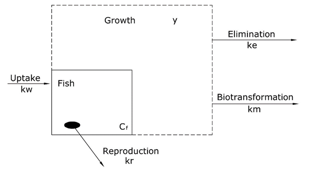
is the uptake rate constant and k2 the elimination rate constant, both with dimension time-1. However, it is often more practical to work with the concentration in the animal (e.g. expressed in mg/kg). This can be achieved by dividing the left and right sides of the equation by w, the body-weight of the animal and defining Cint = Q/w. In addition, we define the external concentration as Cenv = F/V, where V is the volume (L or kg) of the environmental compartment. This leads to the following formulation of the differential equation:


\({dC_{int}\over dt} = k'_1 {V\over w} C_{env} - k_2 C_{int}\)


Beware that Cenv is measured in other units (mg per kg of soil, or mg per litre of water) than Cint (mg per kg of animal tissue). To get rid of the awkward factor V/w it is convenient to define a new rate constant, k1:


\(k_1 = {V\over w} k'_1 \)


This is the uptake rate constant usually reported in scientific papers. Note that it has other units than : it is expressed as kg of soil per kg of animal tissue per time unit (kg kg-1 h-1), and in the case of water exposure as L kg-1 h-1. The dimension of k2 remains the same whether mass or concentrations are used (time-1). We also learn from this analysis that when dealing with concentrations, the body-weight of the animal must remain constant.


References

Moriarty, F. (1984) Persistent contaminants, compartmental models and concentration along food-chains. Ecological Bulletins 36: 35-45.

Skip, B., A.J. Bednarska, & R. Laskowski (2014) Toxicokinetics of metals in terrestrial invertebrates: making things straight with the one-compartment principle. PLoS ONE 9(9): e108740.


Equation 4 describes the whole process with the corresponding graphical representation of the uptake graph (Figure 2).

Figure 2. The basic equation for uptake of a chemical from the aqueous phase to a fish: one compartment model with first order kinetics.


The concentration in the organism is the result of the net process of uptake and elimination. At the initial phase of the accumulation process, elimination is negligible and the ratio of the concentration in the organism is given by:


\({dC_{org} \over dt} = k_w C_{aq}\)                                                                                                   (5)


\(C_{org} (t)= k_w C_{aq} t \)                                                                                              (6)


Steady state

After longer exposure time, elimination becomes more substantial and the uptake curve starts to level off. At some point, the uptake rate equals the elimination rate and the ratio 
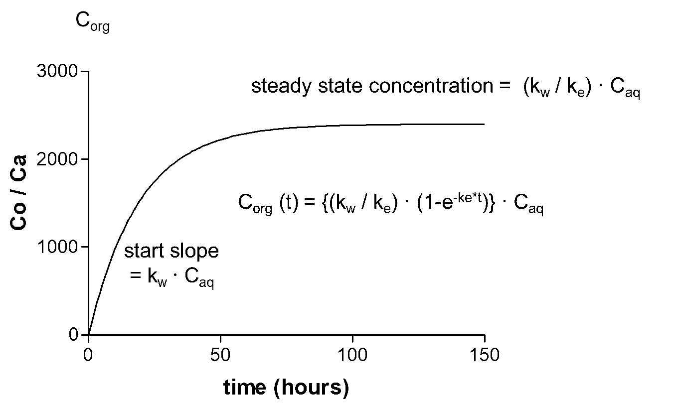
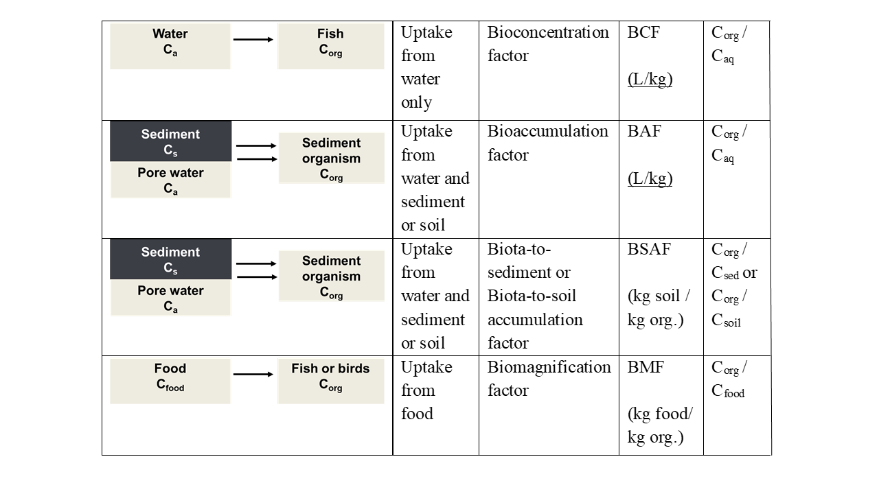
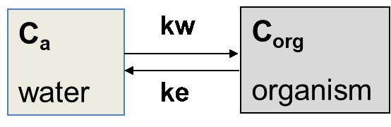
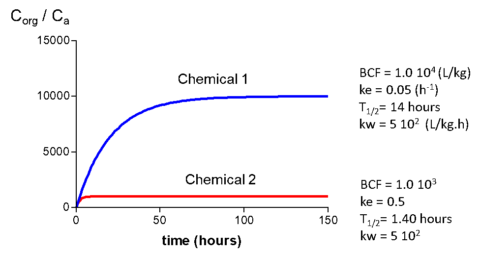
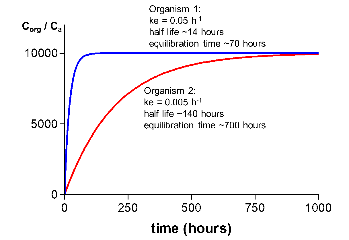
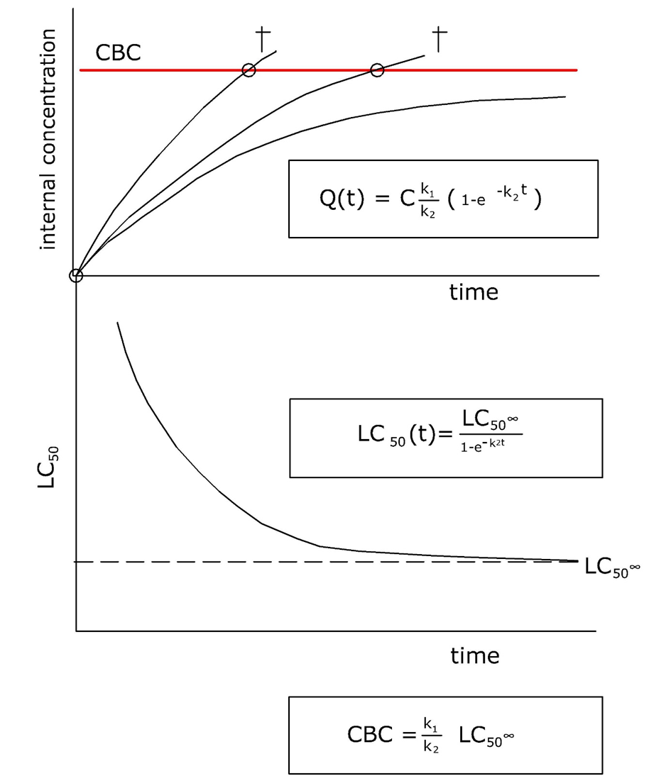
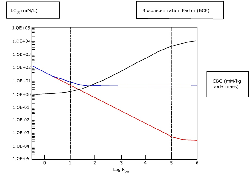
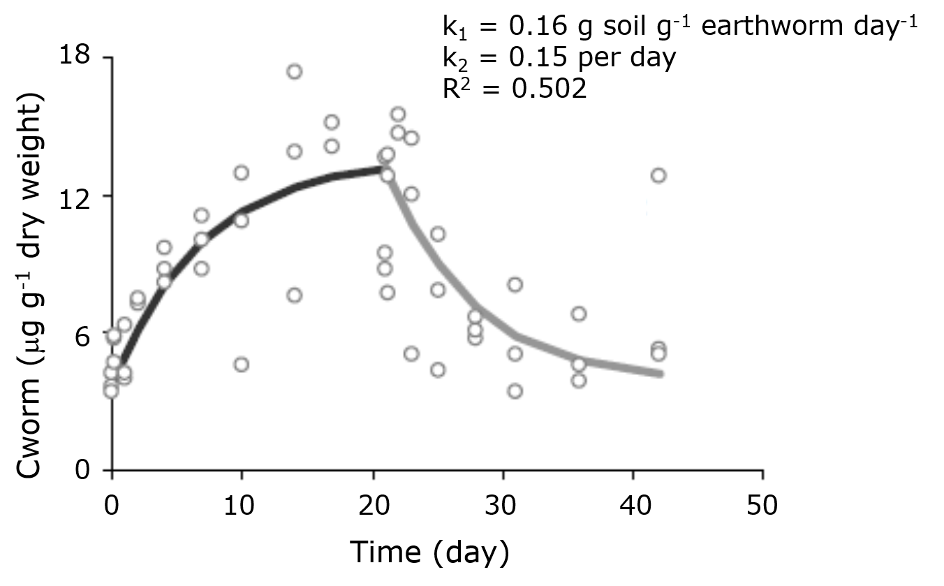
Corg/Caq becomes constant. This is the steady state situation. The constant Corg/Caq at steady state is called the bioconcentration factor BCF. Mathematically, the BCF can also be calculated from kw/ke. This follows directly from equation 4: after long exposure time (t), \( e^{k_e t}\) becomes 0 leading to


\(C_{org} (t)= { k_w \over k_e } C_{aq} \)


\({C_{org} \over C_{aq}} (at\quad steady\quad state) = BCF = {k_w \over k_e} \)                                                           (7)


Elimination

Elimination is often measured following an uptake experiment. After the organism has reached a certain concentration, fish are transferred to a clean environment and concentration in the organism will decrease in time. Because this is also a first order kinetic process, the elimination rate will depend on the concentration in the organism (Corg) and the elimination rate constant (ke) (see equation 8). Concentration will decrease exponentially in time (equation 9) as shown in Figure 3A. Concentrations are often transformed to the natural logarithmic values (ln Corg) because this results in a linear relationship with slope -ke.(equation 10 and figure 3B).


\({dC_{org} \over dt}=- k_e C_{org}\)                                                                                 (8)


\(C_{org} (t)=C_{org} (t=0) e^{-k_e t}\)                                                                (9)


\(ln⁡ C_{org} (t) = ln⁡ C_{org} (t=0) - k_e t\)                                                      (10)


where Corg(t=0) is the concentration in the organism when the elimination phase starts.

The half-life (T1/2 or DT50) is the time needed to eliminate half the amount of chemical from the compartment. The relationship between ke and T1/2 is: T1/2 = (In 2) / ke. The half-life increases when ke decreases.

Figure 3. Elimination of a chemical from fish to water: one compartment model. Left: concentrations given on a normal scale. Right: concentration expressed as the natural logarithm to enable linear regression against time to yield the rate constant as the slope.


Multicompartment models

Very often, organisms cannot be considered as one compartment, but as two or even more compartments (Figure 4A). Deviations from the one-compartment system usually are seen when elimination does not follow an exponential pattern as expected: no linear relationship is obtained after logarithmic transformation. Figure 4B shows the typical trend of the elimination in a two-compartment system. The decrease in concentration (on a logarithmic scale) shows two phases: phase I with a relatively fast decrease and phase II with a relatively slow decrease. According to the linear compartment theory, elimination may be described as the sum of two (or more) exponential terms, like:


\(C_{org} (t) = C_{org} (t=0) F(I) e^{-k_e (I)*t}+F(II)e^{-k_e (II)*t}\)                               (11)


where

ke(I) and ke(II) represent elimination rate constants for compartment I and II,

F(I) and F(II) are the size of the compartments (as fractions)


Typical examples of two compartment systems are:

  • Blood (I) and liver (II)
  • Liver tissue (I) and fat tissue (II)

Elimination from fat tissue is often slower than from, for example, the liver. The liver is a well perfused organ while the exchange between lipid tissue and blood is much less. That explains the faster elimination from the liver.

Figure 4. Elimination of chemical from fish to water (top) in a two-compartment model (bottom).


Examples of uptake curves for different chemicals and organisms

Figure 5 gives uptake curves for two different chemicals and the corresponding kinetic parameters. Chemical 2 has a BCF of 1000, chemical 1 a BCF of 10,000. Uptake rates (kw) are the same, which is often the case for organic chemicals. Half-lives (time to reach 50 % of the steady state level) are 14 and 140 hours. This makes sense because it will take a longer time to reach steady state for a chemical with a higher BCF. Elimination rate constants also differ a factor of 10.

In figure 6, uptake curves are presented for one chemical, but in two organisms of different size/weight. Organism 1 is much smaller than organism 2 and reaches steady state much earlier. T1/2 values for the chemical in organisms 1 and 2 are 14 and 140 hours, respectively. The small size explains this fast equilibration. Rates of uptake depend on the surface-to-volume ratio (S/V) of an organism, which is much higher for a small organism. Therefore, kinetics in small organisms is faster resulting in shorter equilibration times. The effect of size on kinetics is discussed in more detail in Hendriks et al. (2001) and in the Section on Allometric Relationships.

Figure 5. Uptake curves for two chemicals, having different properties, in the same organism.


Figure 6. Uptake curves for the same chemical in two organisms having different sizes; organism 2 is much bigger than organism 1.


Bioaccumulation involving biotransformation and different routes of uptake

In equation 2, elimination only includes gill elimination. If other processes such as biotransformation and growth are considered, the equation can be extended to include these additional processes (see equation 12).


\({dC_{org} \over dt} = k_w C_a-(k_e+ k_m+ k_r ) C_{org} \)                                                      (12)


For organisms living in soil or sediment, different routes of uptake may be of importance: dermal (across the skin), or oral (by ingestion of food and/or soil or sediment particles). Mathematically, the uptake in an organism in sediment can be described as in equation 13.


\(C_{org} (t) = {( k_w C_{aq} + k_s C_s) \over k_e} (1- e^{-k_e t}) \)                                                            (13)


Corg       concentration in organisms (mg/kg)

Caq       concentration in aqueous phase (mg/L)

Cs        concentration soil or sediment (mg/kg)

kw        uptake rate constant from water (L/kg/day)

ks         uptake rate constant from soil or sediment (kgsoil/kgorganism/day)

ke         elimination rate constant (1/day)

t           time (day)

(dimensions used are: amount of chemical: mg; volume of water: L; weight of organism: kg; time: day)


In this equation, kw and ks are the uptake rate constants from water and sediment, ke is the elimination rate constant and Caq and Cs are the concentrations in water and sediment or soil. For soil organisms, such as earthworms, oral uptake appears to become more important with increasing hydrophobicity of the chemical (Jager et al., 2003). This is because the concentration in soil (Cs) will become higher than the porewater concentration Ca for the more hydrophobic chemicals (see section on Sorption).


References

Clewell, H.J., 3rd (1995). The application of physiologically based pharmacokinetic modeling in human health risk assessment of hazardous substances. Toxicology Letters 79, 207-217.

Hendriks, A.J., van der Linde, A., Cornelissen, G., Sijm, D. (2001). The power of size. 1. Rate constants and equilibrium ratios for accumulation of organic substances related to octanol-water partition ratio and species weight. Environmental Toxicology and Chemistry 20, 1399-1420.

Jager, T., Fleuren, R., Hogendoorn, E.A., De Korte, G. (2003). Elucidating the routes of exposure for organic chemicals in the earthworm, Eisenia andrei (Oligochaeta). Environmental Science and Technology 37, 3399-3404.

Nichols, J.W., Fitzsimmons, P.N., Whiteman, F.W. (2004). A physiologically based toxicokinetic model for dietary uptake of hydrophobic organic compounds by fish - II. Simulation of chronic exposure scenarios. Toxicological Sciences 77, 219-229.

Van Leeuwen, C.J., Vermeire, T.G. (Eds.) (2007). Risk Assessment of Chemicals: An Introduction. Springer, Dordrecht, The Netherlands.


4.1.3. Tissue accumulation of metals

Author: Nico M. van Straalen

Reviewers: Philip S. Rainbow, Henk Schat


Learning objectives:

You should be able to

  • indicate four types of inorganic metal binding cellular constituents present in biological tissues and indicate which metals they bind.
  • describe how phytochelatin and metallothionein are induced by metals.
  • mention a number of organ-metal combinations that are critical to metal toxicity.


Key words: Metal binding proteins; phytochelatin; metallothionein;


Synopsis

The issue of metal speciation, which is crucially important to understand metal fate in the environment, is equally important for internal distribution in organisms and toxicity inside the cell. Many metals tend to accumulate in specific organs, for example the hepatopancreas of crustaceans, the chloragogen tissue of annelids, and the kidney of mammals. In addition, there is often a specific organ or tissue where dysfunction or toxicity is first observed, e.g., in the human body, the primary effects of chronic exposure to mercury are seen in the brain, for lead in bone marrow and for cadmium in the kidney. This module is aimed at increasing the insight into the different mechanisms by which metals accumulate in biological tissues.


Introduction

Metals will be present in biological tissues in a large variety of chemical forms: free metal ion, various inorganic species with widely varying solubility, such as chlorides or carbonates, plus all kind of metal species bound to low-molecular and high-molecular weight biotic ligands. The free metal ion is considered the most relevant species relating to toxicity.

To explain the affinities of metals with specific targets, a system has been proposed based on the physical properties of the ion; according to this system, metals are divided into “oxygen-seeking metals” (class A, e.g. lithium, beryllium, calcium and lanthanum), and “sulfur-seeking metals” (class B, e.g. silver, mercury and lead) (See section on Metals and metalloids). However, most of the metals of environmental relevance fall in an intermediate class, called “borderline” (chromium, cadmium, copper, zinc, etc.). This classification is to some extent predictive of the binding of metals to specific cellular targets, such as SH-groups in proteins, nitrogen in histidine or carbonates in bone tissue.

Not only do metals differ enormously in their physicochemical properties, also the organisms themselves differ widely in the way they deal with metals. The type of ligand to which a metal is bound, and how this ligand is transported or stored in the body, determines to a great extent where the metal will accumulate and cause toxicity. Sensitive targets or critical biochemical processes differ between species and this may also lead to differential toxicity.


Inorganic metal binding

Many tissues contain “mineral concretions”, that is, granules with a specific mineral composition that, due to the nature of the mineral, attract different metals. Especially the gut epithelium of invertebrates, and their digestive glands (hepatopancreas, midgut gland, chloragogen tissue) may be full of such concretions. Four classes of granules are distinguished (Figure 1):

  • Calcium-pyrophosphate granules with magnesium, manganese, often also zinc, cadmium, lead and iron
  • Sulfur granules with copper, sometimes also cadmium
  • Iron granules, containing exclusively iron
  • Calcium carbonate granules, containing mostly calcium


Figure 1. Schematic diagram of the gut epithelium of an invertebrate animal, showing four different types of granules and the metals they usually contain. Redrawn from Hopkin (1989) by Wilma IJzerman.


The type B granules are assumed to be lysosomal vesicles that have absorbed metal-loaded peptides such as metallothionein or phytochelatin, and have developed into inorganic granules by degrading almost all organic material; the high sulfur content derives from the cysteine residues in the peptides.

Tissues or cells that specialize in the synthesis of intracellular granules are also the places where metals tend to accumulate. Well-known are the “S cells” in the hepatopancreas of isopods. These cells (small cells, B-type cells sensu Hopkin 1989) contain very large amounts of copper. Most likely the large stores of copper in woodlice and other crustaceans relate to their use of hemocyanin, a copper-dependent protein, as an oxygen-transporting molecule. Similar tissues with high loadings of mineral concretions have been described for earthworms, snails, collembolans and insects.


Organic metal binding

The second class of metal-binding ligands is of organic nature. Many plants but also several animals synthesize a peptide called phytochelatin (PC). This is an oligomer derived from glutathione with the three amino acids, γ-glumatic acid, cysteine and glycine, arranged in the following way: (γ-glu-cys)n-gly, where n can vary from 2 to 11. The thiol groups of several cysteine residues are involved in metal binding.

The other main organic ligand for metals is metallothionein (MT). This is a low-molecular weight protein with hydrophilic properties and an unusually large number of cysteine residues. Several cysteines (usually nine or ten) can bind a number of metal ions (e.g. four or five) in one cluster. There are two such clusters in the vertebrate metallothionein. Metallothioneins occur throughout the tree of life, from bacteria to mammals, but the amino acid sequence, domain structure and metal affinities vary enormously and it is doubtful whether they represent a single evolutionary-homologous group.

In addition to these two specific classes of organic ligands, MT and PC, metals will also bind aspecifically to all kind of cellular constituents, such as cell wall components, albumen in the blood, etc. Often this represents the largest store of metals; such aspecific binding sites will constantly deliver free metal ions to the cellular pool and so are the most important cause of toxicity. Of course metals are also present in molecules with specific metal-dependent functions, such as iron in hemoglobin, copper in hemocyanin, zinc in carbonic anhydrase, etc.

The distinction between inorganic ligands and organic ones is not as strict as it may seem. After binding to metallothionein or phytochelatin metals may be transferred to a more permanent storage compartment, such as the intracellular granules mentioned above, or they may be excreted.


Regulation of metal binding

Free metal ions are strong inducers of stress response pathways. This can be due to the metal ion itself but more often the stress response is triggered by a metal-induced disturbance of the redox state, i.e. an induction of oxidative stress. The stress response often involves the synthesis of metal-binding ligands such as phytochelatin and metallothionein. Because this removes metal ions from the active pool it is also called metal scavenging.

The binding capacity of phytochelatin is enhanced by activation of the enzyme phytochelatin synthase (PC synthase). According to one model of its action, the C-terminus of the enzyme has a “metal sensor” consisting of a number of cysteines with free SH-groups. Any metal ions reacting with this nucleophile center (and cadmium is a strong reactant) will activate the enzyme which then catalyzes the reaction from (γ-glu-cys)n-gly to (γ-glu-cys)n+1-gly, thus increasing the binding capacity of cellular phytochelatin (Figure 2). This reaction of course relies on the presence of sufficient glutathione in the cell. In plants the PC-metal complex is transported into the central vacuole, where it can be stabilized through incorporation of acid-labile sulfur (S2). The PC moiety is degraded, resulting in the formation of inorganic metal-sulfide crystallites. Alternatively, complexes of metals with organic acids may be formed (e.g. citrates or oxalates). The fate of metal-loaded PC in animal cells is not known, but it might be absorbed in the lysosomal system to form B-type granules (see above).


Figure 2. Model for the regulation of phytochelatin synthase, an enzyme catalyzing the extension of phytochelatin and increasing the binding capacity for metals. From Cobbet (2000). Source: http://www.plantphysiol.org/content/123/3/825


The upregulation of metallothionein (MT) occurs in a quite different manner, since it depends on de novo synthesis of the apoprotein. It is a classic example of gene regulation contributing to protection of the cell. In a wide variety of animals, including vertebrates and invertebrates, metallothionein genes (Mt) are activated by a transcription factor called metal-responsive transcription factor 1 (MTF-1). MTF -1 binds to so-called metal-responsive elements (MREs) in the promoter of Mt. MREs are short motives with a characteristic base-pair sequence that form the core of a transcription factor binding site in the DNA. Under normal physiological conditions MTF-1 is inactive and unable to induce Mt. However, it may be activated by Zn2+ ions, which are released, from unspecified ligands, by metals such as cadmium that can replace zinc (Figure 3).


Figure 3. Model for metallothionein induction by cadmium. Cadmium ions (Me) displace zinc ions from ligands (MP). Free zinc ions (Zn) then activate Metal Transcription Factor 1 (MTF-1) in the nucleus to bind to transcription factor binding sites containing Metal-Responsive Elements (MRE). This induces expression of Mt and other genes. These genes may also be induced by oxidative stress, acting upon antioxidant-responsive elements (ARE) and Enhancer Box (E box). Oxidative stress may come from external oxidizing agents or from the metal itself. Finally, zinc ions may also directly activate antioxidant enzymes. Adapted from Haq et al. (2003) by Wilma IJzerman.


It must be emphasized that the model discussed above is inspired by work on vertebrates. Arthropods (Drosophila, Orchesella, Daphnia) could have a similar mechanism since they also have an MTF-1 homolog that activates Mt, however, the situation for other invertebrates such as annelids and gastropods is unclear; their Mt genes seem to lack MREs, despite being inducible by cadmium. In addition, the variability of metallothioneins in invertebrates is extremely large and not all metal-binding proteins may be orthologs of the vertebrate metallothionein. In snails, a cadmium-binding, cadmium-induced MT functions alongside a copper-binding MT while the two MTs have different tissue distributions and are also regulated quite differently.

While both phytochelatin and metallothionein will sequester essential as well as non-essential metals (e.g. Cd) and so contribute to detoxification, the widespread presence of these systems throughout the tree of life suggests that they did not evolve primarily to deal with anthropogenic metal pollution. The very strong inducibility of these systems by non-essential elements like cadmium may be considered a side-effect of a different primary function, for example regulation of the cellular redox state or binding of essential metals.


Target organs

Any tissue-specific accumulation of metals can be explained by turnover of metal-binding ligands. For example, accumulation of cadmium in mammalian kidney is due to the fact that metallothionein loaded with cadmium cannot be excreted. High concentrations of metals in the hind segments of earthworms are due to the presence of “residual bodies” which are fully packed with intracellular granules. Accumulation of cadmium in the human prostrate is due to the high concentration of zinc citrate in this organ, which serves to protect contractile proteins in sperm tails from oxidation; cadmium assumedly enters the prostrate through zinc transporters.

It is often stated that essential metals are subject to regulatory mechanisms, which would imply that their body burden, over a large range of external exposures, is constant. However, not all “essential” metals are regulated to the extent that the whole-body concentration is kept constant. Many invertebrates have body compartments associated with the gut (midgut gland, hepatopancreas, Malpighian tubules) in which metals, often in the form of mineral concretions, are inactivated and stored permanently or exchanged very slowly with the active pool. Since these compartments are outside the reach of regulatory mechanisms but usually not separated in whole-body metal analysis, the body burden as a whole is not constant. Some invertebrates even carry a “backpack” of metals accumulating over life. This holds, e.g., for zinc in barnacles, copper in isopods and zinc in earthworms.

Accumulation of metals in target organs may lead to toxicity when the critical binding or excretion capacity is exhausted and metal ions start binding aspecifically to cellular constituents. The organ in which this happens is often called the target organ. The total metal concentration at which toxicity starts to become apparent is called the critical body concentration (CBC) or critical tissue concentration. For example, the critical concentration for cadmium in kidney, above which renal damage is observed to occur, is estimated to be 50 μg/g. A list of critical organs for metals in the human body is given in Table 1.

The concept of CBC assumes that the complete metal load in an organ is in equilibrium with the active fraction causing toxicity and that there is no permanent storage pool. In the case of storage detoxification the body burden at which toxicity appears will depend on the accumulation history.


Table 1. Critical organs for chronic toxicity of metals in the human body

Metal or metalloid

Critical organ

Symptoms

Al

Brain

Alzheimer’s disease

As

Lung, liver, heart gut

Multisystem energy disturbance

Cd

Kidney, liver

Kidney damage

Cr

Skin, lung, gut

Respiratory system damage

Cu

Liver

Liver damage

Hg

Brain, liver

Mental illness

Ni

Skin, kidney

Allergic reaction, kidney damage

Pb

Bone marrow, blood, brain

Anemia, mental retardation


References

Cobbett, C., Goldsbrough, P. (2002). Phytochelatins and metallothioneins: roles in heavy metal detoxification and homeostasis. Annual Review of Plant Biology 53, 159-182.

Dallinger, R., Berger, B., Hunziker, P., Kägi, J.H.R. (1997). Metallothionein in snail Cd and Cu metabolism. Nature 388, 237-238.

Dallinger, R., Höckner, M. (2013). Evolutionary concepts in ecotoxicology: tracing the genetic background of differential cadmium sensitivities in invertebrate lineages. Ecotoxicology 22, 767-778.

Haq, F., Mahoney, M., Koropatnick, J. (2003) Signaling events for metallothionein induction. Mutation Research 533, 211-226.

Hopkin, S.P. (1989) Ecophysiology of Metals in Terrestrial Invertebrates. London, Elsevier Applied Science.

Nieboer, E., Richardson, D.H.S. (1980) The replacement of the nondescript term "heavy metals" by a biologically and chemically significant classification of metal ions. Environmental Pollution Series B 1, 3-26.

Rainbow, P.S. (2002) Trace metal concentrations in aquatic invertebrates: why and so what? Environmental Pollution 120, 497-507.

4.1.4. Xenobiotic defence and metabolism

Author: Nico M. van Straalen

Reviewers: Timo Hamers, Cristina Fossi


Learning objectives:

You should be able to:

  • recapitulate the phase I, II and III mechanisms for xenobiotic metabolism, and the most important molecular systems involved.
  • describe the fate and the chemical changes of an organic compound that is metabolized by the human body, from absorption to excretion.
  • explain the principle of metabolic activation and why some compounds can become very reactive upon xenobiotic metabolism.
  • develop a hypothesis on the ecological effects of xenobiotic compounds that require metabolic activation.


Keywords: biotransformation; phase 1; phase II; phase III; excretion; metabolic activation; cytochrome P450


Synopsis

All organisms are equipped with metabolic defence mechanisms to deal with foreign compounds. The reactions involved, jointly called biotransformation,  can be divided into three phases, and usually aim to increase water solubility and excretion. The first step (phase I) is catalyzed by cytochrome P450, which is followed by a variety of conjugation reactions (phase II) and excretion (phase III). The enzymes and transporters involved are often highly inducible, i.e. the amount of protein is greatly enhanced by the xenobiotic compounds themselves. The induction involves binding of the compound to cytoplasmic receptor proteins, such as the arylhydrocarbon receptor (AhR), or the constitutive androstane receptor (CAR). In some cases the intermediate metabolites, produced in phase I are extremely reactive and a main cause of toxicity, a well-known example being the metabolic activation of polycyclic aromatic hydrocarbons such as benzo(a)pyrene, which readily forms DNA adducts and causes cancer. In addition, some compounds greatly induce metabolizing enzymes but are hardly degraded by them and cause chronic cellular stress. The various biotransformation reactions are a crucial aspect of both toxicokinetics and toxicodynamics of xenobiotics.


Introduction

The term “xenobiotic” (“foreign to biology”) is generally used to indicate a chemical compound that does not normally have a metabolic function. We will use the term extensively in this module, despite the fact that it is somewhat problematic (e.g., can a compound be considered “foreign” if it circulates in the body, is metabolized or degraded in the body?, and: what is “foreign” for one species is not necessarily “foreign” for another species).

The body has an extensive defence system to deal with xenobiotic compounds, loosely designated as biotransformation. The ultimate result of this system is excretion the compound in some form or another. However, many xenobiotics are quite lipophilic, tend to accumulate and are not easily excreted due to low water solubility. Molecular modifications are usually required before such compounds can be removed from the body, as the main circulatory and excretory systems (blood, urine) are water-based. By introducing hydrophilic groups in the molecule (-OH, =O, -COOH) and by conjugating it to an endogenous compound with good water-solubility, excretion is usually accomplished. However, as we will see below, intermediate metabolites may have enhanced reactivity and it often happens that a compound becomes more toxic while being metabolized. In the case of pesticides, deliberate use is made of such responses, to increase the toxicity of an insecticide once it is in the target organism.

The study of xenobiotic metabolism is a classical subject not only in toxicology but also in pharmacology. The mode of action of a drug often depends critically on the rate and mode of metabolism. Also, many drugs show toxic side-effects as a consequence of metabolism. Finally, xenobiotic metabolism is also studied extensively in entomology, as both toxicity and resistance of pesticides are often mediated by metabolism.

The most problematic xenobiotics are those with a high octanol-water partition coefficient (Kow) that are strongly lipophilic and very hydrophobic. They tend to accumulate, in proportion to their Log Kow, in tissues with a high lipid content such as the subcutis of vertebrates, and may cause tissue damage due to disturbance of membrane functions. This mode of action is called “minimum toxicity”. Well-known are low-molecular weight aliphatic petroleum compounds and chlorinated alkanes such as chloroform. These compounds cause their primary damage to cell membranes; especially neurons are sensitive to this effect, hence minimum toxicity is also called narcotic toxicity. Lipophilic chemicals with high Log Kow do not reach concentrations high enough to cause minimum toxicity because they induce biotransformation at lower concentrations. The toxicity is then usually due to a reactive metabolite.

Xenobiotic metabolism involves three subsequent phases (Figure 1):

  1. Activation (usually oxidation) of the compound by an enzyme known as cytochrome P450, which acts in cooperation with NADPH cytochrome P450 reductase and other factors.
  2. Conjugation of the activated product of phase I to an endogenous compound. A host of different enzymes is available for this task, depending on the compound, the tissue and the species. There are also (slightly polar) compounds that enter phase II directly, without being activated in phase I.
  3. Excretion of the compound into circulation, urine, or other media, usually by means of membrane-spanning transporters belonging to the class of ATP-binding cassette (ABC) transporters, including the infamous multidrug resistance proteins. Hydrophilic compounds may pass on directly to phase III, without being activated or conjugated.


Figure 1. The various phases of xenobiotic metabolism. Redrawn by Wilma Ijzerman.


Phase I reactions

Cytochrome P450 is a membrane-bound enzyme, associated with the smooth endoplasmic reticulum. It carries a porphyrin ring containing an Fe atom, which is the active center of the molecule. The designation P450 is derived from the fact that it shows an absorption maximum at 450 nm when inhibited by carbon monoxide, a now outdated method to demonstrate its presence. Other (outdated) namings are MFO (mixed function oxygenase) and drug metabolizing enzyme complex. Cytochrome P450 is encoded by a gene called CYP, of which there are many paralogs in the genome, all slightly differing from each other in terms of inducibility and substrate specificity. Three classes of CYP genes are involved with biotransformation, designated CYP1, CYP2 and CYP3 in vertebrates. Each class has several isoforms; the human genome has 57 different CYP genes in total. The CYP complement of invertebrates and plants often involves even more genes; many evolutionary lineages have their own set, arising from extensive gene duplications within that lineage. In humans, the genetic complement of a person’s CYP genes is highly relevant as to its drug metabolizing profile (see the section on Genetic variation in toxicant metabolism).

Cytochrome P450 operates in conjunction with an enzyme called NADPH cytochrome P450 reductase, which consists of two flavoproteins, one containing Flavin adenine dinucleotide (FAD), the other flavin mononucleotide (FMN). The reduced Fe2+ atom in cytochrome P450 binds molecular oxygen, and is oxidized to Fe3+ while splitting O2; one O atom is introduced in the substrate, the other reacts with hydrogen to form water. Then the enzyme is reduced by accepting an electron from cytochrome P450 reductase. The overall reaction can be written as:

         RH + O2 + NADPH + H+ → ROH + H2O + NADP+

where R is an arbitrary substrate.


Cytochrome P450 is expressed to a great extent in hepatocytes (liver cells), the liver being the main organ for xenobiotic metabolism in vertebrates (Figure 2), but it is also present in epithelia of the lung and the intestine. In insects the activity is particularly high in the Malpighian tubules in addition to the gut and the fat body. In mollusks and crustaceans the main metabolic organ is the hepatopancreas.


Phase II reactions

After activation by cytochrome P450 the oxidized substrate is ready to be conjugated to an endogenous compound, e.g. a sulphate, glucose, glucuronic acid or glutathione group. These reactions are conducted by a variety of different enzymes, of which some reside in the sER like P450, while others are located in the cytoplasm of the cell (Figure 2). Most of them transfer a hydrophilic group, available from intermediate metabolism, to the substrate, hence the enzymes are called transferases. Usually the compound becomes more polar in phase II, however, not all phase II reactions increase water solubility; for example, methylation (by methyl transferase) decreases reactivity but increases apolarity. Other phase II reactions are conjugation with glutathione, conducted by glutathione-S-transferase (GST) and with glucuronic acid, conducted by UDP-glucuronyl transferase. In invertebrates other conjugations may dominate, e.g. in arthropods and plants, conjugation with malonyl glucose is a common reaction, which is not seen in vertebrates.

Conjugation with glutathione in the human body is often followed by splitting off glutamic acid and glycine, leaving only the cysteine residue on the substrate. Cysteine is subsequently acetylated, thus forming a so-called mercapturic acid. This is the most common type of metabolite for many xenobiotics excreted in urine by humans.

Like cytochrome P450, the phase II enzymes consist in various isoforms, encoded by different paralogs in the genome. Especially the GST family is quite extensive and polymorphisms in these genes contribute significantly to the personal metabolic profile (see the section on Genetic variation in toxicant metabolism).


Figure 2. Schematic view of xenobiotic metabolism (phase I and phase II) in human liver. P450 = cytochrome P450, FP = flavoprotein, RED = cytochrome P450 reductase, EH = epoxide hydrolase, UDP-GT = uridyldiphospho-glucuronyl transferase, GSH-T = glutathione-S-transferase, ST = sulphotransferase. Reproduced from Vermeulen & Van den Broek (1984) by Wilma Ijzerman.


Phase III reactions

In the human body, there are two main pathways for excretion, one from the liver into the bile (and further into the gut and the faeces), the other through the kidney and urine. These two pathways are used by different classes of xenobiotics: very hydrophobic compounds such as high-molecular weight polycyclic aromatic hydrocarbons are still not readily soluble in water even after metabolism but can be emulsified by bile salt and excreted in this way. It sometimes happens that such compounds, once arriving in the gut, are assimilated again, transported to the liver by the portal vein and metabolized again. This is called “entero-hepatic circulation”. Lower molecular weight compounds and hydrophilic compounds are excreted through urine. Volatile compounds can leave the body through the skin and exhaled air.

Excretion of activated and conjugated compounds from tissues out of the cell usually requires active transport, which is mediated by ABC (ATP binding cassette) transporters, a very large and diverse family of membrane proteins which have in common a binding cassette for ATP. Different subgroups of ATP transporters transport different types of chemicals, e.g. positively charged hydrophobic molecules, neutral molecules and water-soluble anionic compounds. One well-known group consists of multidrug resistance proteins or P-glycoproteins. These transporters export drugs aiming to attack tumor cells. Because their activity is highly inducible, these proteins can enhance excretion enormously, making the cell effectively resistant and thus case major problems for cancer treatment.


Induction

All enzymes of xenobiotic metabolism are highly inducible: their activity is normally on a low level but is greatly enhanced in the presence of xenobiotics. This is achieved through a classic case of transcriptional regulation upon CYP and other genes, leading to de novo synthesis of protein. In addition, extensive proliferation of the endoplasmic reticulum may occur, and in extreme cases even swelling of the liver (hepatomegaly).

The best investigated pathway for transcriptional activation of CYP genes is due to the arylhydrocarbon receptor (AhR). Under normal conditions, this peptide is stabilized in the cytoplasm by heat-shock proteins, however, when a xenobiotic compound binds to AhR, it is activated and can join with another protein called Ah receptor nuclear translocator (ARNT) to translocate to the nucleus and bind to DNA elements present in the promotor of CYP and other genes. It thus acts as a transcriptional activator or transcription factor on these genes (Figure 3). The DNA motifs to which AhR binds are called xenobiotic responsive elements (XRE) or dioxin-responsive elements (DRE). The compounds acting in this manner are called 3-MC-type inducers, after the (highly carcinogenic) model compound 3-methylcholanthrene. The inducing capacity of a compound is related to its binding affinity to the AhR, which in itself is determined by the spatial structure of the molecule. The lock-and key fitting between AhR and xenobiotics explains why induction of biotransformation by xenobiotics shows a very strong stereospecificity. For example, among the chlorinated biphenyls and chlorinated dibenzodioxins, some compounds are extremely strong inducers of CYP1 genes, while others, even with the same number of chlorine atoms, are no inducers at all. The precise position of the chlorine atoms determines the molecular “fit” in the Ah receptor (see Section on Receptor interaction).

In addition to 3MC-type of induction there are other modes in which biotransformation enzymes are induced, but these are less well-known. A common class is PB-type induction (named after another model compound, phenobarbital). PB-type induction is not AhR-dependent, but acts through activation of another nuclear receptor, called constitutive androstane receptor (CAR). This receptor activates CYP2 genes and some CYP3 genes.

The high inducibility of biotransformation can be exploited in a reverse manner: if biotransformation is seen to be highly upregulated in a species living in the environment, this indicates that that species is being exposed to xenobiotic compounds. Assays addressing cytochrome P450 activity can therefore be exploited in bioindication and biomonitoring systems. The EROD (ethoxyresorufin-O-deethylase) assay is often used for this purpose, although it is not 100% specific to the isoform of P450. Another approach is to address CYP expression directly, e.g. through reverse transcription-quantitative PCR, a method to quantify the amount of CYP mRNA.


Figure 3. Scheme illustrating how AhR-reactive compounds induce biotransformation activity. 1 xenobiotic compounds enter the cell through diffusion, 2 compound binds to AhR, releasing it from Hsp90, 3 AhR complex is activated by ARNT, 4 translocation to nucleus, 5 binding to XRE, 6 enhanced transcription, 7 translocation of mRNA to cytoplasm and translation, 8 incorporation of P450 enzyme in sER and biotransformation of compounds. AhR = arylhydrocarbon receptor, Hsp90 = heat shock protein 90, ARNT = aryl hydrocarbon nuclear translocator, XRE = xenobiotic responsive element, CYP1 = gene encoding cytochrome P450 1, sER = smooth endoplasmic reticulum. Drawn by Wilma Ijzerman.


Secondary effects of biotransformation

Although the main aim of xenobiotic metabolism is to detoxify and excrete foreign compounds, some pathways of biotransformation actually enhance toxicity. This is mostly due to the first step, activation by cytochrome P450. The activation may lead to intermediate metabolites which are highly reactive and the actual cause of toxicity. The best investigated examples are due to bioactivation of polycyclic aromatic hydrocarbons (PAHs), a group of chemicals present in diesel, soot, cigarette smoke and charred food products. Many of these compounds, e.g. benzo(a)pyrene, benz(a)anthracene and 3-methylcholanthrene, are not reactive or toxic as such but are activated by cytochrome P450 to extremely reactive molecules. Benzo(a)pyrene, for instance, is activated to a diol-epoxide, which readily binds to DNA, especially to the free amino-group of guanine (Figure 4). The complex is called a DNA adduct, the double helix is locally disrupted and this results in a mutation. If this happens in an oncogene, a tumor may develop (see the Section on Carcinogenesis and genotoxicity).

Not all PAHs are carcinogenic. Their activity critically depends on the spatial structure of the molecule, which again determines its “fit” in the Ah receptor. PAHs with a “notch” (often called bay-region) in the molecule tend to be stronger carcinogens than compounds with a symmetric (round or linear) molecular structure.


Figure 4. Metabolism of benzo(a)pyrene (B[a]P) to a mutagenic and carcinogenic metabolite, BaP-diol epoxide. Cytochrome P450 activity (CYP1A1 and CYP1B1) introduces an epoxide on the 7,8 position of the molecule, which is then hydrolyzed by epoxide hydrolase to a dihydrodiol (two OH groups next to each other, which can be in trans position, pointing in different directions relative to the plane of the molecule, or in cis, pointing in the same direction). The trans metabolite is preferably formed. Subsequently another epoxide is introduced on the 9,10 position. The diolepoxide is highly reactive, and may bind proteins and to guanine in DNA, causing a DNA adduct. Modified from Bui et al. (2009) by Steven Droge.


Another mechanism for biotransformation-induced toxicity is due to some very recalcitrant organochlorine compounds such as polychlorinated dibenzodioxins (PCDDs, or dioxins for short) and polychlorinated biphenyls (PCBs). Some of these compounds are very potent inducers of biotransformation, but they are hardly degraded themselves. The consequence is that the highly upregulated cytochrome P450 activity continues to generate a large amount of reactive oxygen (ROS), causing oxidative stress and damage to cellular constituents. It is assumed that the chronic toxicity of 2,3,7,8-tetrachlorodibenzo(para)dioxin (TCDD), one of the most toxic compounds emitted by human activity, is due to its high capacity to induce prolonged oxidative stress. On the molecular level, there is a close link between oxidative stress and biotransformation activity. Many toxicants that primarily induce oxidative stress (e.g. cadmium) also upregulate CYP enzymes. Two defence mechanisms, oxidative stress defence and biotransformation are part of the same integrated stress defence system of the cell.


References

Bui, P.H., Hsu, E.L., Hankinson, O. (2009), Fatty acid hydroperoxides support cytochrome P450 2S1-mediated bioactivation of benzo[a]pyrene-7-8-dihydrodiol. Molecular Pharmacology 76, 1044-1052.

Stroomberg, G.J., Zappey, H., Steen, R.J.C.A., Van Gestel, C.A.M., Ariese, F., Velthorst, N.H., Van Straalen, N.M. (2004). PAH biotransformation in terrestrial invertebrates – a new phase II metabolite in isopods and springtails. Comparative Biochemistry and Physiology Part C 138, 129-137.

Timbrell, J.A. (1982). Principles of Biochemical Toxicology. Taylor & Francis Ltd, London.

Van Straalen, N.M., Roelofs, D. (2012). An Introduction to Ecological Genomics, 2nd Ed. Oxford University Press, Oxford.

Vermeulen, N.P.E., Van den Broek, J.M. (1984). Opname en verwerking van chemicaliën in de mens. Chemisch Magazine. Maart: 167-171.


4.1.5. Allometric relationships

Author: A. Jan Hendriks

Reviewers: Nico van den Brink, Nico van Straalen


Learning objectives:

You should be able to

  • explain why allometrics is important in risk assessment across chemicals and species
  • summarize how biological characteristics such as consumption, lifespan and abundance scale size
  • describe how toxicological quantities such as uptake rates and lethal concentrations scale to size


Keywords: body size, biological properties, scaling, cross-species extrapolation, size-related uptake kinetics


Introduction

Globally more than 100,000,000 chemicals have been registered. In the European Union more than 100,000 compounds are awaiting risk assessment to protect ecosystem and human health, while 1,500,000 contaminated sites potentially require clean-up. Likewise, 8,000,000 species, of which 10,000 are endangered, need protection worldwide, with one lost per hour (Hendriks, 2013). Because of financial, practical and ethical (animal welfare) constraints, empirical studies alone cannot cover so many substances and species, let alone their combinations. Consequently, the traditional approach of ecotoxicological testing is gradually supplemented or replaced by modelling approaches. Environmental chemists and toxicologists for long have developed relationships allowing extrapolation across chemicals. Nowadays, so-called Quantitative Structure Activity Relationships (QSARs) provide accumulation and toxicity estimates for compounds based on their physical-chemical properties. For instance bioaccumulation factors and median lethal concentrations have been related to molecular size and octanol-water partitioning, characteristic properties of a chemical that are usually available from its industrial production process.

In analogy with the QSAR approach in environmental chemistry, the question may be asked whether it is possible to predict toxicological, physiological and ecological characteristics of species from biological traits, especially traits that are easily measured, such as body size. This approach has gone under the name “Quantitative Species Sensitivity Relationships” (QSSR) (Notenboom, 1995).

Among the various traits available, body-size is of particular interest. It is easily measured and a large part of the variability between organisms can be explained from body size, with r2 > 0.5. Not surprisingly, body size also plays an important role in toxicology and pharmacology. For instance, toxic endpoints, such as LC50s, are often expressed per kg body weight. Recommended daily intake values assume a “standard” body weight, often 60 kg. Yet, adult humans can differ in body weight by a factor of 3 and the difference between mouse and human is even larger. Here it will be explored how body-size relationships, which have been studied in comparative biology for a long time, affect the extrapolation in toxicology and can be used to extrapolate between species.


Fundamentals of scaling in biology

Do you expect a 104 kg elephant to eat 104 times more than a 1 kg rabbit per day? Or less, or more? On being asked, most people intuitively come up with the right answer. Indeed, daily consumption by the proboscid is less than 104 times that of the rodent. Consequently, the amount of food or water used per kilogram of body weight of the elephant is less than that of the rabbit. Yet, how much less exactly? And why should sustaining 1 kg of rabbit tissue require more energy than 1 kg of elephant flesh in the first place?

A century of research (Peters, 1983) has demonstrated that many biological characteristics Y scale to size X according to a power function:

Y = a Xb

where the independent variable X represents body mass, and the dependent variable Y can virtually be any characteristic of interest ranging, e.g., from gill area of fish to density of insects in a community.

Plotted in a graph, the equation produces a curved line, increasing super-linearly if b > 1 and sub-linearly if b < 1. If b=1, Y and X are directly proportional and the relationship is called isometric. As curved lines are difficult to interpret, the equation is often simplified by taking the logarithm of the left and right parts. The formula then becomes:

log Y = log a + b log X

When log Y is plotted against log X, a straight line results with slope b and intercept log a. If data are plotted in this way, the slope parameter b may be estimated by simple linear regression.

Across wide size ranges, slope b often turns out to be a multitude of ¼ or, occasionally, ⅓. Rates [kg∙d-1] of consumption, growth, reproduction, survival and what not, increase with mass to the power ¾ , while rate constants, sometimes called specific rates [kg∙kg-1∙d-1], decrease with mass to the power –¼. So, while the elephant is 104 kg heavier than the 1 kg rabbit, it eats only (104)¾ = 103 times more each day. Vice versa, 1 kg of proboscid apparently requires a consumption of (104) kg∙kg-1∙d-1, i.e., 10 times less. Variables with a time dimension [d] like lifespan or predator-prey oscillation periods scale inversely to rate constants and thus change with body mass to the power ¼. So, an elephant becomes (104)¼ = 10 times older than a rabbit. Abundance, i.e., the number of individuals per surface area [m-2] decreases with body mass to the power –¾. Areas, such as gill surface or home range, scale inversely to abundance, typically as body mass to the power ¾.

Now, why would sustaining 1 kg of elephant require 10 times less food than 1 kg of rabbit? Biologists, pharmacologists and toxicologists first attributed this difference to area-volume relationships. If objects of the same shape but different size are compared, the volume increases with length to the power 3 and the surface increases with length to the power 2. For a sphere with radius r, for example, area A and volume V increase as A ~ r2 and V ~ r3, so area scales to volume as A ~ r2 ~ (V)2 ~ V. So, larger animals have relatively smaller surfaces, as long as the shape of the organism remains the same. Since many biological processes, such as oxygen and food uptake or heat loss deal with surfaces, metabolism was, for long, thought to slow down like geometric structures, i.e., with multitudes of ⅓. Yet, empirical regressions, e.g. the “mouse-elephant curve” developed by Max Kleiber in the early 1930s show a universal slope of ¼ (Peters, 1983. This became known as the “Kleiber’s law”. While the data leave little doubt that this is the case, it is not at all clear why it should be ¼ and not ⅓. Several explanations for the ¼ slope have been proposed but the debate on the exact value as well as the underlying mechanism continues.


Application of scaling in toxicology

Since chemical substances are carried by flows of air and water, and inside the organism by sap and blood, toxicokinetics and toxicodynamics are also expected to scale to size. Indeed, data confirm that uptake and elimination rate constants decrease with size, with an exponent of about –¼ (Figure 1). Slopes vary around this value, the more so for regressions that cover small size ranges and physiologically different organisms. The intercept is determined by resistances in unstirred water layers and membranes through which the substances pass, as well as by delays in the flows by which they are carried. The resistances mainly depend on the affinity and molecular size of the chemicals, reflected by, e.g., the octanol-water partition coefficient Kow for organic chemicals or atomic mass for metals. The upper boundary of the intercept is set by the delays imposed by consumption and, subsequently, egestion and excretion. The lower end is determined by growth dilution. Both uptake and elimination scale to mass with the same exponent so that their ratio, reflecting the bioconcentration or biomagnification factor in equilibrium, is independent of body-size.


Figure 1. Regressions of elimination rate constants [kg∙kg-1∙d-1 = d-1] as a function of organism mass m [kg], ranging from algae to mammals, and organic chemicals' octanol-water partition ratio Kow and metal mass within the limits set by consumption and production (redrawn by author, based on Hendriks et al. 2001).


Scaling of rate constants for uptake and elimination, such as in Figure 1, implies that small organisms reach a given internal concentration faster than large ones. Vice versa, lethal concentrations in water or food needed to reach the same internal level after equal (short-term) exposure duration are lower in smaller compared to larger organisms. Thus, the apparent "sensitivity" of daphnids can, at least partially, be attributed to their small body-size. This emphasizes the need to understand simple scaling relationships before developing to more elaborate explanations.

Using Figure 1, one can, within strict conditions not elaborated here, theoretically relate median lethal concentrations LC50 [μg L-1] to the Kow of the chemical and the size of the organism, with r2 > 0.8 (Hendriks, 1995; Table 1). Complicated responses like susceptibility to toxicants can be predicted only from Kow and body size, which illustrates the generality and power of allometric scaling. Of course, the regressions describe the general trends and in individual cases the deviations can be large. Still, considering the challenges of risk assessment as outlined above, and in the absence of specific data, the predictions in Table 1 can be considered as a reasonable first approximation.


Table 1. Lethal concentrations and doses as a function of test animal body-mass

Species

Endpoint

Unit

b (95% CI)

r2

nc

ns

Source

Guppy

LC50

mg∙L-1

0.66 (0.51-0.80)

0.98

6

1

1

Mammals

LD10≈MTD

mg∙animal-1

0.73

0.69‑0.77

27

5

2

Birds

Oral LD50

mg∙animal-1

1.19 (0.67-0.82)

0.76

194

3…37

3

Mammals

Oral LD50

mg∙animal-1

0.94 (1.18-1.20)

0.89

167

3…16

4

Mammals

Oral LD50

mg∙animal-1

1.01 (1.00-1.01)


>5000

2…8

5

MTD = maximum threshold dose, repeated dosing. LD50 single dose, b = slope of regression line, nc = number of chemicals, ns = number of species. Sources: 1 Anderson & Weber (1975), 2 Travis & White (1987), 4 Sample & Arenal (1999), 5 Burzala-Kowalczyk & Jongbloed (2011).


Allometry is also important when dealing with other levels of biological organisation. Leaf or gill area, the number of eggs in ovaries, the number of cell types and many other cellular and organ characteristics scale to body-size as well. Likewise, intrinsic rates of increase (r) of populations and the production-biomass ratios (P/B) of communities can also be obtained from the (average) species mass. Even the area needed by animals in laboratory assays scales to size, i.e., by m¾, approximately the same slope noted for home ranges of individuals in the field.


Future perspectives

Since almost any physiological and ecological process in toxicokinetics and toxicodynamics depends on species size, allometric models are gaining interest. Such an approach allows one to quantitatively attribute outliers (like apparently "sensitive" daphnids) to simple biological traits, rather than detailed chemical-toxicological mechanisms.

Scaling has been used in risk assessment at the molecular level for a long time. The molecular size of a compound is often a descriptor in QSARs for accumulation and toxicity. If not immediately evident as molecular mass, volume or area often pops up as an indicator of steric properties. Scaling does not only apply to bioaccumulation and toxicity from molecular to community levels, size dependence is also observed in other sections of the environmental cause-effect chain. Emissions of substances, e.g., scale non-linearly to the size of engines and cities. Concentrations of chemicals in rivers depend on water discharge, which in itself is an allometric function of catchment size. Hence, understanding the principles of cross-disciplinary scaling is likely to pay off in protecting many species against many chemicals.


References

Anderson, P.D., Weber, L.J. (1975). Toxic response as a quantitative function of body size. Toxicology and Applied Pharmacology 33, 471-483.

Burzala-Kowalczyk, L., Jongbloed, G. (2011). Allometric scaling: Analysis of LD50 data. Risk Analysis 31, 523-532.

Hendriks, A.J. (1995). Modelling response of species to microcontaminants: Comparative ecotoxicology by (sub)lethal body burdens as a function of species size and octanol-water partitioning of chemicals. Ecotoxicology and Environmental Safety 32, 103-130.

Hendriks, A.J. (2013). How to deal with 100,000+ substances, sites, and species: Overarching principles in environmental risk assessment. Environmental Science and Technology 47, 3546−3547.

Hendriks, A.J., Van der Linde, A., Cornelissen, G., Sijm, D.T.H.M. (2001). The power of size: 1. Rate constants and equilibrium ratios for accumulation of organic substances. Environmental Toxicology and Chemistry 20, 1399-1420.

Notenboom, J., Vaal, M.A., Hoekstra, J.A. (1995). Using comparative ecotoxicology to develop quantitative species sensitivity relationships (QSSR). Environmental Science and Pollution Research 2, 242-243.

Peters, R.H. (1983). The Ecological Implications of Body Size. Cambridge University Press, Cambridge.

Sample, B.E., Arenal, C.A. (1999) Allometric models for interspecies extrapolation of wildlife toxicity data. Bulletin of Environmental Contamination and Toxicology 62, 653-66.

Travis, C.C., White, R.K. (1988) Interspecific scaling of toxicity data. Risk Analysis 8, 119-125.

4.1.6. Food chain transfer

Auteur: Nico van den Brink

Reviewers: Kees van Gestel. Jan Hendriks


Learning objectives:

You should be able to:

  • Mention the chemical properties determining the potential of chemicals to accumulate in food chains
  • Explain the role of biological and ecological factors in the food-chain accumulation of chemicals


Keywords: biomagnification, food-chain transfer,


Accumulation of chemicals across different trophic levels.

Chemicals may be transferred from one organism to another. Grazers will ingest chemicals that are in the vegetation they eat. Similarly, predators are exposed to chemicals in their prey items. This so-called food web accumulation is governed by properties of the chemical, but also by some traits of the receiving organism (e.g. grazer or predator).


Chemical properties driving food web accumulation

Some chemicals are known to accumulate in food webs, reaching the highest concentrations in top-predators. Examples of such chemicals are organochlorine pesticides like DDT and brominated flame retardants (e.g. PBDEs; see section on POPs). Such accumulating chemicals have a few properties in common: they need to be persistent and they need to have affinity for the organismal body. Organic chemicals with a relatively high log Kow, indicating a high affinity for lipids, will enter organisms quite effectively (see section on Bioconcentration and kinetics modelling). Once in the body, these chemicals will be distributed to lipid rich tissues, and excretion is rather limited. In case of persistent chemicals that are not metabolised, concentrations will increase over time when uptake is higher than excretion. Furthermore, such chemicals are likely to be passed on to organisms at the next trophic level in case of prey-predator interactions. Some of these chemicals may be metabolised by the organism, most often into more water soluble metabolites (see section on Xenobiotic metabolism & defence). These metabolites are more easily excreted, and in this way concentrations of metabolizable chemicals do not increase so much over time, and will therefore also transfer less to higher trophic levels. The effects of metabolism on the internal concentrations of organisms is clearly illustrated by a study on the uptake of organic chemicals by different aquatic species (Kwok et al., 2013). In that study the uptake of persistent chemicals (organochlorine pesticides; OCPs) was compared with the uptake of chemicals that may be metabolised (polycyclic aromatic hydrocarbons; PAHs). The authors compared shrimps with fish, the former having a limited capacity to metabolise PAHs while fish can. Figure 1 shows the Biota-to-Sediment Accumulation Factors (BSAFs; see section on Bioaccumulation), which is the ratio between the concentration in the organism and in the sediment. It is shown that OCPs accumulate to a high extent in both species, reflecting persistent, non-metabolizable chemicals. For PAHs the results are different per species, fish are able to metabolise and as a result the concentrations of PAHs in the fish are low, while in shrimp, with a limited metabolic capacity, the accumulation of PAHs is comparable to the OCPs. These results show that not only the properties of the chemicals are of importance, but also some traits of the organisms involved, in this case the metabolic capacity.


Figure 1. Biota–sediment accumulation factors organochlorine pesticides (OCPs) and polycyclic aromatic hydrocarbons (PAHs) in fish and shrimp. Redrawn from Kwok et al. (2013).


Effects of species traits and food web structure on food web accumulation

Food-web accumulation of chemicals is driven by food uptake. At lower trophic levels, most organisms will acquire relatively low concentrations from the ambient environment. First consumers, foraging on these organisms will accumulate the chemicals of all of them, and in case of persistent chemicals that enter the body easily, concentrations in the consumers will be higher than in their diet. Similarly, concentrations will increase when the chemicals are transferred to the next trophic level. This process is called biomagnification, indicating increasing concentrations of persistent and accumulative chemicals in food webs. The most iconic example of this is on the increasing concentrations of DDTs in fish eating American Osprey (Figure 2), a casus which has led to the ban of a lot of organochlorine chemicals.


Figure 2. Example of biomagnification of DDT in an aquatic food web of ospreys. Slightly modified from: http://naturalresources.anthro-seminars.net/concepts/ecological-concepts-biomagnification/.


Since biomagnification along trophic levels is food driven, it is of importance to include diet composition into the studies. This can be explained by an example on small mammals in the Netherlands. Two similar small mammal species, the bank vole (Myodes glareolus) and the common vole (Microtus arvalis) co-occur in larger part of the Netherlands. Although the species look very similar, they are different in their diet and habitat use. The bank vole is a omnivorous species, inhabiting different types of habitat while the common vole is strictly vegetarian living in pastures. In a study on the species-specific uptake of cadmium, diet items of both species were analysed, indicating nearly 3 orders of magnitudes differences in cadmium concentrations between earthworms and berries from vegetation (Fig 3A, van den Brink et al., 2010). Stable isotopic ratios of carbon and nitrogen were used to assess the general diets of the organisms. The common vole ate mostly stinging nettle and grass, including seeds, while the bank vole showed to forage on grass herbs and earthworms. This difference in diet was reflected in increased concentrations of cadmium in the bank vole in comparison to the common vole (both inhabiting the same area). The concentrations of one bank vole appeared to be extremely low (red diamond in Figure 3b), and initially this was considered to be an artefact. However, detailed analysis of the stable isotopic ratios in this individual revealed that it had foraged on stinging nettle and grass, hence a diet more reflecting the common vole. This emphasises once more that organisms accumulate through their diet (you accumulate what you eat!)


Figure 3. Left: Concentrations of cadmium in diet items of small mammals collected in the Plateaux area near Eindhoven, the Netherlands; Right: Cadmium concentrations in kidneys of bank voles and common voles collected in the Plateaux area. See text for further explanation. Redrawn from van den Brink et al. (2010).


Case studies

Orcas or Killer whales (Orcinus orca) are large marine predatory mammals, which roam all around the oceans, from the Arctic to the deep south region of the Antarctic. Although they appear ubiquitous around the world, generally different pods of Orcas occur in different regions of the marine ecosystem. Often, each pod has developed specialised foraging behaviours targeted at specific prey species. Although Orcas are generally apex top-predators at the top of the (local) food web, the different foraging strategies would suggest that exposure to accumulating chemicals may differ considerably between pods. This was indeed shown to be the case in a very elaborate study on different pods of Orcas of the West-coast of Canada by Ross et al. (2000). In the Vancouver region there is a resident pod while the region is also often visited by two transient groups of Orcas. PCB concentrations were high in all animals, but the transient animals contained significantly higher levels. The transient whales mainly fed on marine mammals, while the resident animals mainly fed on fish, and this difference in diet was thought to be the cause of the differences in PCB levels between the groups. In that study, it was also shown that PCB levels increased with age, due to the persistence of the PCBs, while female orcas contained significant lower concentrations of PCBs. The latter is caused by the lactation of the female Orcas during which they feed their calves with lipid rich milk, containing relatively high levels of (lipophilic) PCBs. By this process, females offload large parts of their PCB body burden, however by transferring these PCBs to their developing calves (see also Figure 3 in the section on Bioaccumulation). A recent study showed that although PCBs have been banned for decades now, they still pose threats to populations of Orcas (Deforges et al., 2018). In that study, regional differences in PCB burdens were confirmed, likely due to differences in diet preferences although not specifically mentioned. It was shown that PCB levels in most of the Orca populations were still above toxic threshold levels and concerns were raised regarding the viability of these populations. This study confirms that 1) Orcas are exposed to different levels of PCBs according to their diet, which influences the biomagnification of the PCBs, 2) Orca populations are very inefficient in clearing PCBs from the individual due to little metabolism but also from the population due to the efficient maternal transfer from mother to calve, and 3) persistent, accumulating chemicals may pose threats to organisms even decades after their use. Understanding the mechanisms and processes underlying the biomagnification of persistent and toxic compounds is essential for a in depth risk assessment.


References

Desforges, J.-P., Hall, A., McConnell, B., Rosing-Asvid, A., Barber, J.L., Brownlow, A., De Guise, S., Eulaers, I., Jepson, P.D., Letcher, R.J., Levin, M., Ross, P.S., Samarra, F., Víkingson, G., Sonne, C., Dietz, R. (2018). Predicting global killer whale population collapse from PCB pollution. Science 361, 1373-1376.

Ford, J.K.B., Ellis, G.A., Matkin, D.R., Balcomb, K.C., Briggs, D., Morton, A.B. (2005). Killer whale attacks on minke whales: Prey capture and antipredator tactics. Marine Mammal Science 21, 603-618.

Guinet, C. (1992). Predation behaviour of killer whales (Orcinus orca) around Grozet Islands. Canadian Journal of Zoology 70, 1656-1667.

Kwok, C.K., Liang, Y., Leung, S.Y., Wang, H., Dong, Y.H., Young, L., Giesy, J.P., Wong, M.H. (2013). Biota–sediment accumulation factor (BSAF), bioaccumulation factor (BAF), and contaminant levels in prey fish to indicate the extent of PAHs and OCPs contamination in eggs of waterbirds. Environmental Science and Pollution Research 20, 8425-8434.

Ross, P.S., Ellis, G.M., Ikonomou, M.G., Barrett-Lennard, L.G., Addison, R.F. (2000). High PCB concentrations in free-ranging Pacific killer whales, Orcinus orca: Effects of age, sex and dietary preference. Marine Pollution Bulletin 40, 504-515.

Samarra, F.I.P., Bassoi, M., Beesau, J., Eliasdottir, M.O., Gunnarsson, K., Mrusczok, M.T., Rasmussen, M., Rempel, J.N., Thorvaldsson, B., Vikingsson, G.A. (2018). Prey of killer whales (Orcinus orca) in Iceland. Plos One 13, 20.

van den Brink, N., Lammertsma, D., Dimmers, W., Boerwinkel, M.-C., van der Hout, A. (2010). Effects of soil properties on food web accumulation of heavy metals to the wood mouse (Apodemus sylvaticus). Environmental Pollution 158, 245-251.


4.1.7. Critical Body Concentration

Author: Martina G. Vijver

Reviewers: Kees van Gestel and Frank Gobas


Learning objectives:

You should be able to

  • describe the Critical Body Concentration (CBC) concept for assessing the toxicity of chemicals.
  • graphically explain the CBC concept and make a distinction between slow and fast kinetics.
  • mention cases in which the CBC approach fails.


Keywords:

Time dependent effects, internal body concentrations, one compartment model


Introduction

One of the quests in ecotoxicology is how to link toxicity to exposure and to understand why some organisms experience toxic effects while others do not at the same level of exposure. A generally accepted approach for assessing possible adverse effects on biota, no matter what kind of species, is the Critical Body Concentration (CBC) concept (McCarty 1991). According to this concept, toxicity is determined by the amount of chemical taken up, so by the internal concentration, which has a relationship with the duration of the exposure as well as the exposure concentration.

Figure 1 shows the relationship between the development with time of the internal concentrations of a chemical in an organism and the time when mortality occurs at different exposure concentrations under constant exposure. Independent of exposure time or exposure concentration, mortality occurs at a more or less fixed internal concentration. The CBC is defined as the highest internal concentration of a substance in an organism that does cause a defined effect, e.g. 50% mortality or 50% reduction in the number of offspring produced. By comparing internal concentrations measured in exposed organisms to CBC values derived in the laboratory, a measure of risk is obtained. The CBC applies to lethality as well as to sub-lethal effects like reproduction or growth inhibition.


Relating toxicity to toxicokinetics

From Figure 1A, it may also become clear that chemicals that have fast uptake kinetics will reach the CBC faster than chemicals that have slow kinetics (see Section on Bioaccumulation kinetics). As a consequence, also the time to reach a constant LC50 (indicated as the ultimate LC50: LC50¥; Figure 1B) depends on kinetics. Hence, both toxic effects and chemical concentration are controlled by the same kinetics.The CBC can be derived from the LC50-time relationship and be linked to the LC50¥ using uptake and elimination rate constants (k1 and k2). It should be noted that the k2 in this case does not reflect the rate of chemical excretion but rather the rate of elimination of toxic effects caused by the chemical (so, note the difference here with Section on Bioaccumulation kinetics).


Figure 1: A. The relationship between uptake kinetics of a chemical in an organism and its toxicity according to the Critical Body Concentration (CBC) concept under constant exposure. The red line depicts the highest internal concentration of the chemical in the organism killing the organism (CBC); exceedance of that line results in mortality. B. The relationship between LC50 and time. LC50 will reach a constant value with time, indicated as the ultimate LC50 (LC50¥). The CBC can be calculated from the LC50¥ using uptake and elimination rate constants (k1 and k2) derived by first order kinetics as shown here. Note: the CBC approach is not limited to first order kinetics. And the same curves may be seen when focusing on sublethal effects, LC50 then reads EC50. Drawn by Wilma Ijzerman.


The time needed to reach steady state depends on the body size of the organisms, with larger organisms taking longer time to attain steady state compared to smaller organisms (McCarty 1991). The time needed to reach steady state depends also on the exposure surface area of the exposed organisms (Pawlisz and Peters 1993) as well as their metabolic activity. Organisms not capable of excreting or metabolizing a chemical will continue accumulating with time, and the LC50¥ will be zero. This is e.g. the case for cadmium in isopods (Crommentuijn et al. 1994), but kinetics are so slow that cadmium in these animals never reaches lethal concentrations in relatively clean environments as their life span is too short.

The CBC integrates environmentally available fractions with bioavailable concentrations and toxicity at specific receptors (McCarty and MacKay 1993). See also Section on Bioavailability. In this way, the actual exposure concentration in the environment does not need to be known for performing a risk assessment. The internal concentration of the chemical in the organism is the only concentration required for a risk assessment. Therefore many difficulties are overcome regarding bioavailability issues, e.g. it removes some of the disadvantages of the exposure concentration expressed per unit of soil, as well as of dealing with exposures that vary over time or space.


Proof of the CBC concept

A convincing body of evidence was collected to support the CBC approach. For organic compounds with a narcotic mode of action, effects could be assessed over a wide range of organisms, test compounds and exposure media. For narcotic compounds with octanol-water partition coefficients (Kow) varying from 10 to 1,000,000 (see for details Section on Relevant chemical properties), the concentration of chemical required for lethality through narcosis is approximately 1-10 mmol/kg: Figure 2 (McCarty and MacKay 1993).


Figure 2: Theoretical plot supporting the Critical Body Concentration (CBC) concept for non-polar organic chemicals acting by narcosis. The bioconcentration factor (BCF in L/kg body mass; black line) of these chemicals increases with increasing log Kow while their acute toxicity also increases (LC50 in test solution in mM decreases; red line). The product of LC50 and BCF is the critical body concentrations (in mM/kg body mass; blue line). Adapted from McCarty and Mackay (1993) by Wilma Ijzerman.


To reduce the variation in bioconcentration factor (BCF) values for the accumulation of chemicals in organisms from water, normalization by lipid content has been suggested allowing to determine the chemical activity within an organism’s body (US EPA 2003). For that reason, lipid extraction protocols are intensively described within the updated OECD Guideline for the testing of chemicals No. 305 for fish bioaccumulation tests, along with a sampling schedule of lipid measurement in fish. Correction of the BCF for differences in lipid content is also described in the same OECD guideline No. 305. If chemical and lipid analyses have been conducted on the same fish, this requires correction for the corresponding lipid content of each individual measured concentration in the fish. This should be done prior to using the data to calculate the kinetic BCF. If lipid content is not measure on all sampled fish, a mean lipid content of approx. 5% must be used to normalize the BCF. It should be noted that this correction holds only for chemicals accumulating in lipids and not for chemicals that do primarily bind to proteins (e.g. perfluorinated substances).


When does the CBC concept not apply?

The CBC concept also has some limitations. Crommentuijn et al. (1994) found that the toxicity of metals to soil invertebrates could not be explained using critical body concentrations. The way different organisms deal with accumulated metals has a large impact on the magnitude of body concentrations reached and the accompanying metal sensitivity (Rainbow 2002). Moreover, adaptation or development of metal tolerance limits the application of CBCs for metals. When the internal metal concentration does not show a monotonic relationship with the exposure concentration, it is not possible to derive CBCs. This means that whenever organisms are capable of trapping a portion of the metal in forms that are not biologically reactive, a direct relationship between body metal concentrations and toxicity may be absent or less evident (Luoma and Rainbow 2005, Vijver et al. 2004). Consequently, for metals a wide range of body concentrations with different biological significance exists. It therefore remains an open question whether the approach is applicable to modes of toxic action other than narcosis. Another important point is the question to what extent the CBC approach is applicable to assessing the effect of chemical mixtures, especially in cases the chemicals have a different mode of action.


References

Crommentuijn, T., Doodeman, C.J.A.M., Doornekamp, A., Van der Pol, J.J.C., Bedaux, J.J.M., Van Gestel, C.A.M. (1994). Lethal body concentrations and accumulation patterns determine time-dependent toxicity of cadmium in soil arthropods. Environmental Toxicology and Chemistry 13, 1781-1789.

Luoma, S.N., Rainbow, P.S. (2005). Why is metal bioaccumulation so variable? Biodynamics as a unifying concept. Environmental Science and Technology 39, 1921-1931

McCarty, L.S. (1991). Toxicant body residues: implications for aquatic bioassays with some organic chemicals. In: Mayes, M.A., Barron, M.G. (Eds.), Aquatic Toxicology and Risk Assessment: Fourteenth Volume. ASTM STP 1124. Philadelphia: American Society for Testing and Materials. pp. 183-192. DOI: 10.1520/STP23572S

McCarty, L.S., Mackay, D. (1993). Enhancing ecotoxicological modeling and assessment. Environmental Science and Technology 27, 1719-1727

Pawlisz, A.V., Peters, R.H. (1993). A test of the equipotency of internal burdens of nine narcotic chemicals using Daphnia magna. Environmental Science and Technology 27, 2801-2806

Rainbow P.S. (2002). Trace metal concentrations in aquatic invertebrates: why and so what? Environmental Pollution 120, 497-507.

U.S. EPA. (2003). In: Methodology for Deriving Ambient Water Quality Criteria for the Protection of Human Health: Technical Support Document. Volume 2. United States Environmental Protection Agency, Washington, D.C: Development of National Bioaccumulation Factors.

Vijver M.G., Van Gestel, C.A.M., Lanno, R.P., Van Straalen, N.M., Peijnenburg, W.J.G.M. (2004) Internal metal sequestration and its ecotoxicological relevance: a review. Environmental Science and Technology 18, 4705-4712.

4.2. Toxicodynamics & Molecular Interactions

Author: Timo Hamers

Reviewers: Frank van Belleghem and Ludek Blaha


Learning goals

You should be able to

  • explain that a toxic response requires a molecular interaction between a toxic compound and its target
  • name at least three different types of biomolecular targets
  • name at least three functions of proteins that can be hampered by toxic compounds
  • explain in general terms the consequences of molecular interaction with a receptor protein, an enzyme, a transporter protein, a DNA molecule, and a membrane lipid bilayer.


Key words: Receptor; Transcription factor; DNA adducts; Membrane; Oxidative stress


Description

Toxicodynamics describes the dynamic interactions between a compound and its biological target, leading ultimately to an (adverse) effect. In this Chapter 4.2, toxicodynamics have been described for processes leading to diverse adverse effects. Any adverse effects by a toxic substance is the result of an interaction between the toxicant and its biomolecular target (i.e. mechanism of action). Biomolecular targets include a protein, a DNA or RNA molecule, a phospholipid bilayer membrane, but also small molecules that have specific functions in keeping cellular homeostasis.


Both endogenous and xenobiotic compounds that bind to proteins are called ligands. The consequence of a protein interaction depends on the role of the target protein, e.g.

1. Receptor

2. Enzyme

3. Protein

Receptor proteins specifically bind and respond to endogenous signalling ligands such as hormones, prostaglandins, growth factors, or neurotransmitters, by causing a typical cellular response. Receptor proteins can be located in the cell membrane, in the cytosol, and in the nucleus of a cell. Agonistic receptor ligands activate the receptor protein whereas antagonistic ligands inactivate the receptor and prevent (endogenous) agonists from activating the receptor. Based on the role of the receptor protein, binding by ligands may interfere with ion channels, G-protein coupled receptors, enzyme linked receptors, or nuclear receptors.  Xenobiotic ligands can interfere with these cellular responses by acting as agonistic or antagonistic ligands (link to section on Receptor interaction).


Compounds that bind to an enzyme usually cause inhibition of the enzyme activity, i.e. a decrease in the conversion rate of the endogenous substrate(s) of the enzyme into its/their corresponding product(s). Compounds that bind non-covalently to an enzyme cause reversible inhibition, while compounds that bind covalently to an enzyme cause irreversible inhibition (link to section on Protein inactivation).


Similarly, compounds that bind to a transporter protein usually inhibit the transport of the natural, endogenous ligand. Such transporter proteins may be responsible for local transport of endogenous ligands across the cell membrane, but also for peripheral transport of endogenous ligands through the blood from one organ to the other (link to section Endocrine disruption).


Apart from interaction with functional receptor, enzyme, or transporter proteins, toxic compounds may also interact with structural proteins. For instance the cytoskeleton may be damaged by toxic compounds that block the polymerization of actin, thereby preventing the formation of filaments.


In addition to proteins, DNA and RNA macromolecules can be targets for compound binding. Especially the guanine base can be covalently bound by electrophilic compounds, such as reactive metabolites. Such DNA adducts may cause copy errors during  DNA replication leading to point mutations (link to section on Genotoxicity).


Compounds may also interfere with phospholipid bilayer membranes, especially with the outer cell membrane and with mitochondrial membranes. Compounds disturb the membrane integrity and functioning by partitioning into the lipid bilayer. Lost membrane integrity may ultimately lead to leakage of electrolytes and loss of membrane potential.


Narcosis and Membrane Damage

Partitioning into the lipid bilayer is a non-specific process. Therefore, concentrations in biological membranes that cause effects through this mode of action do not differ between compounds. As such, this type of toxicity is considered as a “baseline toxicity” (also called “narcosis”), which is exerted by all chemicals. For instance, the chemical concentration in a target membrane causing 50% mortality in a test population is around 50 mmol/kg lipid, irrespective of the species or compound under consideration. Based on external exposure levels, however, compounds do have different narcotic potencies. After all, to reach similar lipid-based internal concentrations, different exposure concentrations are required, depending on the lipid-water partitioning coefficient, which is an intrinsic property of a compound, and not of the species.


Narcotic action is not the only mechanism by which compounds may damage membrane integrity. Compounds called “ionophores”, for instance, act like ion carriers that transport ions across the membrane, thereby disrupting the electrolyte gradient across the membrane. Ionophores should not be confused with compounds that open or close ion channels, although both type of compounds may disrupt the electrolyte gradient across the membrane. The difference is that ionophores dissolve in the bilayer membrane and shuttle transport ions across the membrane themselves, whereas ion channel inhibitors or stimulators close or open, respectively, a protein channel in the membrane that acts as a gate for ion transport.


Finally, it should be mentioned here that some compounds may cause oxidative stress  by increasing the formation of reactive oxygen species (ROS), such as H2O2, O3, O2•-, •OH, NO•, or RO•. ROS are oxygen metabolites that are found in any aerobic living organism. Compounds may directly cause an increase in ROS formation by undergoing redox cycling or interfering with the electron transport chain. Alternatively, compounds may cause an indirect increase in ROS formation by interference with ROS-scavenging antioxidants, ranging from small molecules (e.g. glutathione) to proteins (e.g. catalase or superoxide dismutase). For compounds causing both direct or indirect oxidative stress, it is not the compound itself that has a molecular interaction with the target, but the ROS which may bind covalently to DNA, proteins, and lipids (link to section on Oxidative Stress).


4.2.1. Protein Inactivation

Author: Timo Hamers

Reviewers: Frank van Belleghem and Ludek Blaha


Learning objectives:

You should be able to

  • discuss how a compound that binds to a protein may inhibit ligand binding, and thereby hamper the function of the protein
  • explain the mechanism of action of organophosphate insecticides inhibiting acetylcholinesterase
  • explain the mechanism of action of halogenated phenols inhibiting thyroid hormone transport by transthyretin
  • distinguish between reversible and irreversible protein inactivation
  • distinguish between competitive, non-competitive, and uncompetitive enzyme inhibition


Key words: enzyme inhibition; acetylcholinesterase, transthyretin, competitive inhibition, non-competitive inhibition, uncompetitive inhibition


Introduction

Proteins play an important role in essential biochemical processes including catalysis of metabolic reactions, DNA replication and repair, transport of messengers (e.g. hormones), or receptor responses to such messengers. Many toxic compounds exert their toxic action by binding to a protein and thereby disturbing these vital protein functions.


Inhibition of the protein transport function

Binding of xenobiotic compounds to a transporter protein may hamper binding of the natural ligand of the protein, thereby inhibiting the transporter function of the protein. An example of such inhibition is the binding of halogenated phenols to transthyretin (TTR). TTR is a transport protein for thyroid hormones, present in the blood. It has two binding places for the transport of thyroid hormone, i.e. mainly thyroxine (T4) in mammals and mainly triiodothyronine (T3)  in other vertebrates (Figure 1). Compounds with high structural resemblance with thyroid hormone (especially halogenated phenols, such as hydroxylated metabolites of PCBs or PBDEs), are capable to compete with thyroid hormone for TTR binding. Apart from the fact that this enhances distribution of the toxic compounds, this also causes an increase of unbound thyroid hormone in the blood, which is then freely available for uptake in the liver, metabolic conjugation, and urinary excretion. Ultimately, this may lead to decreased thyroid hormone levels in the blood.


Figure 1: Structural resemblance between T4, a hydroxylated PCB metabolite (4-OH-CB-107) and a hydroxylated PBDE metabolite (3-OH-BDE-47). The lower panel illustrates how halogenated phenols (red; e.g. OH-PCB), given their structural resemblance with T4, can compete with T4 (cyan) for TTR-binding (pink), thereby increasing the levels of unbound T4.


Inhibition of the protein enzymatic activity

Proteins involved in the catalysis of a metabolic reaction are called enzymes. The general formula of such a reaction is

Binding of a toxic compound to an enzyme usually causes an inhibition of the enzyme activity, i.e. a decrease in the conversion rate of the endogenous substrate(s) of the enzyme into its/their corresponding product(s). In practice, this causes a toxic response due to a surplus of substrate and/or a deficit of product. One of the classical examples of enzyme inhibition by toxic compounds is the inhibition of the enzyme acetylcholinesterase (AChE) by organophosphate insecticides. AChE catalyzes the hydrolysis of the neurotransmitter acetylcholine (ACh), in the cholinergic synapses. During transfer of an action potential from one cell to the other, ACh is released in these synapses from the presynaptic cell into the synaptic cleft in order to stimulate the acetylcholine-receptor (AChR) on the membrane of the postsynaptic cell. AChE, which is also present in these synapses, is then responsible to break down the ACh into acetic acid and choline:


By covalent binding to serine residues in the active site of the AChE enzyme, organophosphate insecticides can inhibit this reaction causing accumulation of the ACh neurotransmitter in the synapse (Fig. 2). As a consequence, the AChR is overstimulated causing convulsions, hypertension, muscle weakness, salivation, lacrimation, gastrointestinal problems, and slow heartbeat.


Figure 2: ACh (blue) is released from the presynaptic neuron into the synapse where it merges to and activates the AChR present on membrane of the postsynaptic cell (not shown). Meanwhile, AChE (grey) present in the synaptic cleft hydrolyses the ACh neurotransmitter to avoid overstimulation of the postsynaptic membrane. Organophosphate insecticides (red) bind to the AChE and prevent its reaction with ACh, causing accumulation of ACh.


Irreversible vs reversible enzyme inhibition

Organophosphate insecticides bind covalently to the AChE enzyme thereby causing irreversible enzyme inhibition. Irreversible enzyme inhibition progressively increases in time following first-order kinetics (link to section on Bioaccumulation and kinetic modelling). Recovery of enzyme activity can only be obtained by de novo synthesis of enzymes. In contrast to AChE inhibition,  inhibition of the T4 transport function of TTR is reversible because the halogenated phenols bind to TTR in a non-covalent way. Similarly, non-covalent binding of a toxic compound to an enzyme causes reversible inhibition of the enzyme activity.


In addition to covalent and non-covalent enzyme binding, irreversible enzyme inhibition may occur when toxic compounds cause an error during enzyme synthesis. For instance, ions of essential metals, which are present as cofactors in the active site of many enzymes, may be replaced by ions of other metals during enzyme synthesis, yielding inactive enzymes. A classic example of such decreased enzyme activity is the inhibition of δ-aminolevulinic acid dehydratase (δ-ALAD) by lead. In this case, lead replaces zinc in the active site of the enzyme, thereby inhibiting a catalytic step in the synthesis of a precursor of heme, a cofactor of the protein hemoglobulin (link to section on Toxicity mechanisms of metals).


With respect to reversible enzyme inhibition, three types of inhibition can be distinguished, i.e. competitive, non-competitive, and uncompetitive inhibition (Figure 3).


Figure 3: Three types of reversible enzyme inhibition, i.e. competitive (left), non-competitive (middle), and uncompetitive (right) binding.  See text for further explanation. Source: juang.bst.ntu.edu.tw/files/Enz04%20inhibition.PPT


Competitive inhibition refers to a situation where the chemical competes (“fights”) with the substrate for binding to the active site of the enzyme. Competitive inhibition is very specific, because it requires that the inhibitor resembles the substrate and fits in the same binding pocket of the active site. The TTR-binding example described above is a typical example of competitive inhibition between thyroid hormone and halogenated phenols for occupation of the TTR-binding site. A more classic example of competitive inhibition is the inhibition of beta-lactamase by penicillin. Beta-lactamase is an enzyme responsible for the hydrolysis of beta-lactam, which is the final step in bacterial cell wall synthesis. By defective cell wall synthesis, penicillin is an antibiotic causing bacterial death.

Non-competitive inhibition refers to a situation where the chemical binds to an allosteric site of the enzyme (i.e. not the active site), thereby causing a conformational change of the active site. As a consequence, the substrate cannot enter the active site, or the active site becomes inactive, or the product cannot be released from the active site. For instance, echinocandin antifungal drugs non-competitively inhibit the enzyme 1,3-beta glucan synthase, which is responsible for the synthesis of beta-glucan, a major constituent of the fungal cell wall. Lack of beta-glucan in fungal cell walls prevents fungal resistance against osmotic forces, leading to cell lysis.

Uncompetitive inhibition refers to a situation where the chemical can only bind to the enzyme if the substrate is simultaneously bound. Substrate binding leads to a conformational change of the enzyme, which leads to the formation of an allosteric binding site for the inhibitor. Uncompetitive inhibition is more common in two-substrate enzyme reactions than in one-substrate enzyme reactions. An example of uncompetitive inhibition is the inhibition by lithium of the enzyme inositol mono phosphatase (IMPase), which is involved in recycling of the second messenger inositol-3-phospate (I3P) (link to section on Receptor interaction). IMPase is involved in the final step of dephosphorylating inositol monophosphate into inositol. Since lithium is the primary treatment for bipolar disorder, this observation has led to the inositol depletion hypothesis that inhibition of inositol phosphate metabolism offers a plausible explanation for the therapeutic effects of lithium.

4.2.2. Receptor interaction

Author: Timo Hamers

Reviewers: Frank van Belleghem and Ludek Blaha


Learning objectives

You should be able to

  • explain the possible effects of compound interference with ion channels.
  • explain the possible effects of compound interference with G-protein coupled receptors (GPCRs).
  • explain the possible effects of compound interference with enzyme linked receptors.
  • explain the possible effects of compound interference with nuclear receptors.
  • understand what signalling pathways are and how they can be affected to toxic compounds


Key words: Ion channels, G-protein coupled receptors, enzyme linked receptors, nuclear receptors


Introduction

Receptor proteins specifically bind and respond to endogenous signalling ligands such as hormones, prostaglandins, growth factors, or neurotransmitters, by causing a typical cellular response. Receptor proteins can be located in the cell membrane, in the cytosol, and in the nucleus of a cell. Agonistic receptor ligands activate the receptor protein whereas antagonistic ligands inactivate the receptor and prevent (endogenous) agonists from activating the receptor (Figure 1). Based on the role of the receptor protein, binding by ligands may interfere with:

1. ion channels

2. G-protein coupled receptors

3. enzyme-linked receptors

4. nuclear receptors.

Xenobiotic ligands can interfere with these cellular responses by acting as agonistic or antagonistic ligands.

.

Figure 1: Activation by the endogenous ligand of a receptor leads to an effect. An agonistic compound may also activate the receptor and leads in cooperation with the endogenous ligand to an enhanced effect. An antagonistic compound also has binding affinity for the receptor, but cannot activate it. Instead, it prevents the endogenous ligand from binding, and activating the receptor, thereby preventing the effect.


1. Ion channels

Ion channels are transmembrane protein complexes that transport ions across a phospholipid bilayer membrane. Ion channels are especially important in neurotransmission, when stimulating neurotransmitters (e.g. acetylcholine or ACh) bind to the (so-called ionotropic) receptor part of the ion channel and open the ion channel for a very short (i.e. millisecond) period of time. As a result, ions can cross the membrane causing a change in transmembrane potential (Figure 2). On the other hand, receptor-binding by inhibiting neurotransmitters (e.g. gamma-aminobutyric acid or GABA) prevents the opening of ion channels.


Figure 2. The acetylcholine receptor (AChR) is a sodium channel. During neurotransmission from the presynaptic to the postsynaptic cell, binding of the neurotransmitter acetylcholine (ACh) to AChR causes opening of the sodium channel allowing depolarisation of the postsynaptic membrane and propagation of the action potential. Drawn by Evelin Karsten-Meessen.


Compounds interfering with sodium channels, for instance, are neurotoxic compounds (see section on Neurotoxicity). They can either block the ion channels or keep them in a prolonged or permanently open state. Many compounds known to interfere with ion channels are natural toxins. For instance, tetrodotoxin (TTX), which is produced by marine bacteria and highly accumulated in puffer fish, and saxitoxin, which is produced by dinoflagellates and is accumulated in shellfish are capable of blocking voltage-gated sodium channels in nerve cells. In contrast, ciguatoxin, which is another persistent toxin produced by dinoflagellates that accumulates in predatory fish positioned high in the food chain, causes prolongation of the opening of voltage-gated sodium channels. Some pesticides like DDT and pyrethroid insecticides also prevent closure of voltage-gated sodium channels in nerve cells. As a consequence, full repolarization of the membrane potential is not achieved. As a consequence, the nerve cells do not reach the resting potential and any new stimulus that would be too low to reach the threshold for depolarization under normal conditions, will now cause a new action potential. In other words, the nerve cells become hyperexcitable and undergo a series of action potentials (repetitive firing) causing tremors and hyperthermia.


2. G-protein coupled receptors (GPCRs)

GPCRs are transmembrane receptors that transfer an extracellular signal into an activated G-protein that is connected to the receptor on the intracellular side of the membrane. G-proteins are heterotrimer proteins consisting of three subunits alpha, beta, and gamma, of which the alpha subunit – in inactivated form – contains a guanosine diphosphate (GDP) molecule. Upon binding by endogenous ligands such as hormones, prostaglandins, or neurotransmitters (i.e. the signal or “first messenger”) to the (so-called metabotropic) receptor, a conformational change in the GPCR complex leads to an exchange of the GDP for a guanosine triphosphate (GTP) molecule in the alpha monomer part of the G-protein, causing release of the activated alpha subunit from the beta/gamma dimer part. The activated alpha monomer can interact with several target enzymes causing an increase in “second messengers” starting signal transduction pathways (see point 3 Enzyme-linked receptors). The remaining beta-gamma complex may also move along the inner membrane surface and affect the activity of other proteins (Figure 3).


Figure 3. Mechanism of GPCR-activation: ligand binding causes a conformational change leading to the release of an activated alpha monomer, which interacts with a target enzyme (causing an increase of second messengers), and a beta-gamma dimer, which may directly affect activity of other proteins (e.g. an ion channel). Source: http://courses.washington.edu/conj/bess/gpcr/gpcr.htm


Two major enzymes that are activated by the alpha monomer are adenylyl cyclase causing an increase in second messenger cyclic AMP (cAMP) and phospholipase C causing an increase in second messenger diacylglycerol (DAG). In turn, cAMP and DAG activate protein kinases, which can phosphorylate many other enzymes. Activated phospholipase C also causes an increase in levels of the second messenger inositol-3-phosphate (I3P), which opens ion channels in the endoplasmic reticulum causing a release of calcium from the endoplasmic store, which also acts as a second messenger.  On the other hand, the increase in cytosolic calcium levels is simultaneously tempered by the beta/gamma dimer, which can inhibit voltage-gated calcium channels in the cell membrane. Ultimately, the GPCR signal is extinguished by slow dephosphorylation of GTP into GDP by the activated alpha monomer, causing it to rearrange with the beta/gamma dimer into the original inactivated trimer G-protein (see also https://courses.washington.edu/conj/bess/gpcr/gpcr.htm).

The most well-known example of disruption of GPCR signalling is by cholera toxin (see text block Cholera toxin below).

Despite the recognized importance of GPRCs in medicine and pharmacology, little attention has so-far been paid in toxicology to interaction of xenobiotics with GPCRs. Although a limited number of studies have demonstrated that endocrine disrupting compounds including PAHs, dioxins, phthalates, bisphenol-A, and DDT can interact with GPCR signalling, the toxicological implications of these interactions (especially with respect to disturbed energetic metabolism) remain subject for further research (see review by Le Ferrec and Øvrevik, 2018).


Cholera toxin

Cholera toxin is a so-called AB exotoxin by Vibrio cholerae bacteria, consisting of an “active” A-part and a “binding” B-part (see http://www.sumanasinc.com/webcontent/animations/content/diphtheria.html). Upon binding by the B-part to the intestinal epithelium membrane, the entire AB complex is internalized into the cell via endocytosis, and the active A-part is released. This A-part adds an ADP-ribose group to G-proteins making the GTP dephosphorylation of activated G-proteins impossible. As a consequence, activated G-proteins remain in a permanent active state, adenylyl cyclase is permanently activated and cAMP levels rise, which in turn cause an imbalance in ion housekeeping, i.e. an excessive secretion of chloride ions to the gut lumen and a decreased uptake of sodium ions from the gut lumen. Due to the increased osmotic pressure, water is released to the gut lumen causing dehydration and severe diarrhoea (“rice-water stool”).


3. Enzyme-linked receptors

Enzyme-linked receptors are transmembrane receptors that transfer an extracellular signal into an intracellular enzymatic activity. Most enzyme-linked receptors belong to the family of receptor tyrosine kinase (RTK) proteins. Upon binding by endogenous ligands such as hormones, cytokines, or growth factors (i.e. the signal or primary messenger) to the extracellular domain of the receptors, the receptor monomers dimerize and develop kinase activity, i.e. become capable of coupling of a phosphate group donated by a high-energy donor molecule to an acceptor protein. The first substrate for this phosphorylation activity is the dimerized receptor itself, which accepts a phosphate group donated by ATP on its intracellular tyrosine residues. This autophosphorylation is the first step of a signalling pathway consisting of a cascade of subsequent phosphorylation steps of other kinase proteins (i.e. signal transduction), ultimately leading to transcriptional activation of genes followed by a cellular response (Figure 4).


Figure 4. Upon ligand binding, tyrosine kinase receptor (TKR) proteins become autophosphorylated and may phosphorylate (i.e. activate other proteins), including other kinases. Drawn by Evelin Karsten-Meessen.


Xenobiotic compounds can interfere with these signalling pathways in many different ways. Compounds may avoid binding of the endogenous ligand,  by blocking the receptor or by chelating the endogenous ligands. Most RTK inhibitors inhibit the kinase activity directly by acting as a competitive inhibitor for ATP binding to the tyrosine residues. Many RTK inhibitors are used in cancer treatment, because RTK overactivity is typical for many types of cancer. This overactivity may for instance be caused by increased levels of receptor-activating growth factors, or to spontaneous dimerization when the receptor is overexpressed or mutated).


4. Nuclear receptors

Nuclear receptors are proteins that are activated by endogenous compounds (often hormones) leading ultimately to expression of genes specifically regulated by these receptors. Apart from ligand binding, activation of most nuclear receptors requires dimerization with a coactivating transcription factor. While some nuclear receptors are located in the nucleus in inactive form (e.g. the thyroid hormone receptor), most nuclear receptors are located in the cytosol, where they are bound to co-repressor proteins (often heat-shock proteins) keeping them in an inactive state. Upon ligand binding to the ligand binding domain (LBD) of the receptor, the co-repressor proteins are released and the receptor either forms a homodimer with a similar activated nuclear receptor or forms a heterodimer with a different nuclear receptor, which is often the retinoid-X receptor (RXR) for nuclear hormone receptors. Before or after dimerization, activated nuclear receptors are translocated to the nucleus. In the nucleus, they bind through their DNA-binding domain (DBD, or “zinc finger”) to a responsive element in the DNA located in the promotor region of receptor-responsive genes. Consequently, these genes are transcribed to mRNA in the nucleus, which is further translated into proteins in the cell cytoplasm, see Figure 5).


Figure 5. Activation of a cytosolic nuclear receptor (NR). Upon ligand binding (e.g. a hormone), the heat shock proteins (HSP) dissociate from the ligand-receptor complex, which forms a heterodimer before entering the nucleus. After recruiting other coactivating transcription factors, the activated dimer binds to the hormone response element (HRE). RNA polymerase binds to this complex and starts transcription of mRNA, which is excreted from the nucleus into the cytosol and transcribed in corresponding proteins. Source: https://upload.wikimedia.org/wikipedia/commons/3/3f/Nuclear_receptor_action.png


Xenobiotic compounds may act as agonist or antagonists of nuclear receptor activation. Chemicals that act as a nuclear receptor agonist mimic the action of the endogenous activator(s), whereas chemicals that act as a nuclear receptor antagonist basically block the LBD of the receptor, preventing the  binding of the endogenous activator(s). Over the past decades, interaction of xenobiotics with nuclear receptors involved in signalling of both steroid and non-steroid hormones has gained a lot of attention of researchers investigating endocrine disruption (link to section on Endocrine Disruption). Nuclear receptor activation is also the key mechanism in dioxin-like toxicity (see text block dioxin-like toxicity below).


Dioxin-like toxicity

The term dioxins refers to polyhalogenated dibenzo-[p]-dioxin (PHDD) compounds, which are planar molecules consisting of two halogenated aromatic rings, which are connected by two ether bridges. The most potent and well-studied dioxin is 2,3,7,8-tetrachloro-[p]-dibenzodioxin (2,3,7,8-TCDD), which is often too simply referred to as TCDD or even just “dioxin”. Other compounds with similar properties (dioxin-like compounds) include polyhalogenated dibenzo-[p]-furan (PHDF) compounds (often too simply referred to as “furans”), which are planar molecules consisting of two halogenated aromatic rings connected by one ether bridge and one carbon-carbon bond. A third major class of dioxin-like compounds belong to the polyhalogenated biphenyls (PHB), which consist of two halogenated aromatic rings connected only by a carbon-carbon bond. The most well-known compounds belonging to this latter category are the polychlorinated biphenyls (PCBs). Of all PHDD, PHDF or PHB compounds, only the persistent and planar compounds are considered dioxin-like compounds. For the PHBs, this implies that they should contain zero or at maximum one halogen-substitution in any of the four ortho-positions (see examples below). Non-ortho-substituted PHBs can easily obtain a planar confirmation with the two aromatic rings in one planar field, whereas mono-ortho-substituted PHBs can obtain such confirmation at higher energetic costs..

2,3,7,8-tetrachlorodibenzo-[p]-dioxin (2,3,7,8-TCDD) is the most potent and well-studied dioxin-like compound, usually too simply referred to as “dioxin”.

2,3,7,8-tetrachlorodibenzo-[p]-furan (2,3,7,8-TCDF) a dioxin-like compound equally potent to 2,3,7,8-TCDD. It is usually too simply referred to as “furan”.

3,3’,4,4’,5-pentachlorinated biphenyl (PCB-126) is the most potent dioxin-like PCB compound, with no chlorine substitution in any of the four ortho positions next to the carbon-carbon bridge

2,3’,4,4’,5-pentachlorinated biphenyl (PCB-118) is a weak  dioxin-like PCB compound, with one chlorine substitution in the four ortho positions next to the carbon-carbon bridge

2,2’,4,4’,5,5’-hexachlorinated biphenyl (PCB-153) is a non-dioxin-like (NDL) PCB compound, with two chlorine substitution in the four ortho positions next to the carbon-carbon bridge


The planar composition is required for the dioxin-like compounds to fit as a key in the lock of the arylhydrocarbon (AhR) receptor (also known as the “dioxin-receptor or DR), present in the cytosol. The activated AhR then dissociates from its repressor proteins, is translocated to the nucleus, and forms a heterodimer with the AhR nuclear translocator (ARNT). The AhR-ARNT complex binds to dioxin-response elements (DRE) in the promotor regions of dioxin-responsive genes in the DNA, ultimately leading to transcription and translation of these genes (Figure 6). Famous examples of such genes belong to the CYP1, UGT, and GST families, which are Phase I and Phase II metabolic enzymes whose activation by the AhR-ARNT complex is a natural response triggered by the need to remove xenobiotics (link to section on Xenobiotic metabolism and defence). Other genes with a DRE in their promotor region include genes involved in protein phosphorylation, such as the proto-oncogen c-raf and the cyclin dependent kinase inhibitor p27.


Figure 6. Classical mechanism of induction of gene expression by compounds interacting with the arylhydrocarbon receptor (AhR). The AhR is present in the cytosol as a complex with two heat shock proteins (hsp90), X-associated protein 2 (XAP2). Upon ligand binding by polyhalogenated aromatic hydrocarbons (see text) the complex is transferred to the nucleus, where the activated AhR first dissociates from its chaperone proteins and then forms a dimer with the AhR nuclear translocator (ARNT). Upon binding of the dimer to dioxin responsive elements (DREs) in the DNA, dioxin-responsive genes (such as cytochrome P-4501A1 or CYP1A1) or transcribed and translated. Redrawn from Denison and Nagy (2003) by by Evelin Karsten-Meessen.


This classical mechanism of ligand:AhR:ARNT:DRE complex-dependent induction of gene expression, however, cannot explain all the different types of toxicity observed for dioxins, including immunotoxicity, reproductive toxicity and developmental toxicity. Still, these effects are known to be mediated through the AhR as well, as they were not observed in AhR knockout mice. This can partly be explained by the fact that not all genes that are under transcriptional control of a DRE are known yet. Moreover, AhR dependent mechanisms other than this classical mechanism have been described. For instance, AhR activation may have anti-estrogenic effects because activated AhR (1) binds to the estrogen receptor (ER) and targets it for degradation, (2) binds (with ARNT) to inhibitory DREs in the promotor of ER-dependent genes, and (3) competes with the ER-dimer for common coactivators.  Although dioxin-like compounds absolutely require the AhR to exert their major toxicological effects, several AhR independent effects have been described as well, such as AhR-independent alterations in gene expression and changes in Ca2+ influx related to changes in protein kinase activity.


Apart from the persistent halogenated dioxinlike compounds described above, other compounds may also activate the AhR, including natural AhR agonists (nAhRAs) found in food (e.g. indolo[3,2-b]carbazole (ICZ) in cruciferous vegetables, bergamottin in grapefruits, tangeretin in citrus fruits), and other planar aromatic compounds, including polycyclic aromatic hydrocarbons (PAHs) produced by incomplete combustion of organic fuels. Upon activation of the AhR, these non-persistent compounds are metabolized by the induced CYP1A biotransformation enzymes. In addition, an endogenous AhR ligand called 6-formylindolo[3,2-b]carbazole (FICZ) has been identified. FICZ is a mediator in many physiological processes, including immune responses, cell growth and differentiation. Endogenous FICZ levels are regulated by a negative feedback FICZ/AhR/CYP1A loop, i.e. FICZ activates AhR and is metabolized by the subsequently induced CYP1A. Dysregulation of this negative feedback loop by other AhR agonists may disrupt FICZ functioning, and could possibly explain some of the effects observed for dioxinlike compounds.


Further reading:

Denison, M.S., Soshilov, A.A., He, G., De Groot, D.E., Zhao, B. (2011). Exactly the same but different: promiscuity and diversity in the molecular mechanisms of action of the Aryl hydrocarbon (Dioxin) Receptor. Toxicological Sciences 124, 1-22.


Further reading:

Boelsterli, U.A. (2009). Mechanistic Toxicology (2nd edition). Informa Healthcare, New York, London.

Denison, M.S., Nagy, S.R. (2003). Activation of the aryl hydrocarbon receptor by structurally diverse exogenous and endogenous chemicals. Annual Reviews of Pharmacology and Toxicology 43, 309–334.

Le Ferrec, E., Øvrevik J. (2018). G-protein coupled receptors (GPCR) and environmental exposure. Consequences for cell metabolism using the b-adrenoceptors as example. Current Opinion in Toxicology 8, 14-19.

https://courses.washington.edu/conj/bess/gpcr/gpcr.htm


4.2.3. Oxidative stress - I.

Reactive oxygen species and antioxidants


Author: Frank van Belleghem

Reviewers: Raymond Niesink, Kees van Gestel, Éva Hideg


Learning objectives:

You should be able to

  • explain what oxidative stress is, under which circumstances it arises and why it is important in toxicology.
  • describe what reactive oxygen species are and how they are produced.
  • describe how levels of reactive oxygen species are kept under control.
  • make a distinction between enzymatic and non-enzymatic antioxidants.


Keywords: Reactive oxygen species, Fenton reaction, Enzymatic antioxidants, Non-enzymatic antioxidants, Lipid peroxidation.


Reactive oxygen species

Molecular oxygen (O2) is a byproduct of photosynthesis and essential to all heterotrophic cells because it functions as the terminal electron acceptor during the oxidation of organic substances in aerobic respiration. This process results in the reduction of O2 to water, leading to the formation of chemical energy and reducing power. The reason why O2 can be reduced with relative ease in biological systems can be found in the physicochemical properties of the oxygen molecule (in the triplet ground state, i.e. as it occurs in the atmosphere). Because of its electron configuration, O2 is actually a biradical that can act as an electron acceptor. The outer molecular orbitals of O2 each contain one electron, the spins of these electrons are parallel (Figure 1). As a result, oxygen (in the ground state) is not very reactive because, according to the Pauli exclusion principle, only one electron at a time can react with other electrons in a covalent bond. As a consequence, oxygen can only undergo univalent reductions, and the complete reduction of oxygen to water requires the sequential addition of four electrons leading to the formation of one-, two-, three-electron oxygen intermediates (Figure 1). These oxygen intermediates are, in sequence, the superoxide anion radical (O2●-), hydrogen peroxide (H2O2) and the hydroxyl radical (OH).

Another reactive oxygen species of importance is singlet oxygen (1O2 or 1Δg). Singlet oxygen is formed by converting ground-state molecular oxygen into an excited energy state, which is much more reactive than the normal ground-state molecular oxygen. Singlet oxygen is typically generated by a process called photosensitization, for example in the lens of the eye. Photosensitization occurs when light (UV) absorption by an endogenous or xenobiotic substance lifts the compound to a higher energy state (a high-energy triplet intermediate) which can transfer its energy to oxygen, forming highly reactive singlet oxygen. Apart from oxygen-dependent photodynamic reactions, singlet oxygen is also produced by neutrophils and this has been suggested to be important for bacterial killing through the formation of ozone (O3) (Onyango, 2016).  

Because these oxygen intermediates are potentially deleterious products that can damage cellular components, they are referred to as reactive oxygen species (ROS). ROS are also often termed ‘free radicals’ but this is incorrect because not all ROS are radicals (e.g. H2O2, 1O2 and O3). Moreover, as all radicals are (currently) considered as unattached, the prefix ‘free’ is actually unnecessary (Koppenol & Traynham, 1996).


Figure 1. Consecutive four-step one-electron reduction of oxygen yielding reactive oxygen intermediates and 2 H2O. Step 1 is superoxide anion radical generation by acceptance of one electron. This step is endothermic and hence rate-limiting. The next steps are exothermic and hence spontaneous. In step 2, the superoxide anion radical is reduced by acceptance of one electron and protonated by two H+, resulting in H2O2 formation. In step 3, H2O2 undergoes heterolytic fission in which one oxygen atom receives both electrons from the broken covalent bond. This moiety is protonated yielding one molecule H2O. The other moiety receives one electron (generated by the Fenton reaction, see text) and is transformed into a hydroxyl free radical (OH). In step 4,OH receives one electron, and after protonation, yields one molecule H2O. Figure adapted from Edreva (2005) by Steven Droge.


ROS are byproducts of aerobic metabolism in the different organelles of cells, for instance respiration or photosynthesis, or as part of defenses against pathogens. Endogenous sources of reactive oxygen species include oxidative phosphorylation, P450 metabolism, peroxisomes and inflammatory cell activation. For example, superoxide anion radicals are endogenously formed from the reduction of oxygen by the semiquinone of ubiquinone (coenzyme Q), a coenzyme widely distributed in plants, animals, and microorganisms. Ubiquinones function in conjunction with enzymes in cellular respiration (i.e., oxidation-reduction processes). The superoxide anion radical is formed when one electron is taken up by one of the antibonding π*-orbitals (formed by two 2p atomic orbitals) of molecular oxygen.


Figure 2. A simplified representation of the reaction of the semiquinone anion radical with molecular oxygen to form the superoxide anion radical. Figure adapted from Bolton & Dunlap (2016) by Steven Droge.


A second example of an endogenous source of superoxide anion radicals is the auto-oxidation of reduced heme proteins. It is known, for example, that oxyferrocytochrome P-450 substrate complexes may undergo auto-oxidation and subsequently split into (ferri) cytochrome P-450, a superoxide anion radical and the substrate (S). This process is known as the uncoupling of the cytochrome P-450 (CYP) cycle and also referred to as the oxidase activity of cytochrome P-450. However, it should be mentioned that this is not the normal functioning of CYP. Only when the transfer of an oxygen atom to a substrate is not tightly coupled to NADPH utilization, so that electrons derived from NADPH are transferred to oxygen to produce O2●- (and also H2O2).

Table 1 shows the key oxygen species and their biological half-life, their migration distance, the endogenous source and their reaction with biological compounds.


Table 1. The key oxygen species and their characteristics (table adapted from Das & Roychoudhury, 2014)

ROS species

Half-life (T1/2)

Migration distance

Endogenous source

Mode of action

Superoxide anion radical (O2●-)

1-4 µs

30 nm

Mitochondria, cytochrome P450, macrophage/ inflammatory cells, membranes, chloroplasts

Reacts with compounds with double bonds

Hydroxyl radical (OH)

1 µs

1 nm

Mitochondria, membranes, chloroplasts

Reacts vigorously with all biomolecules.

Hydrogen peroxide (H2O2)

1 ms

1 µm

Mitochondria, membranes,

peroxisomes, chloroplasts

Oxidizes proteins by reacting with the Cys residue.

Singlet Oxygen

1-4 µs

30 nm

Mitochondria, membranes, chloroplasts

Oxidizes proteins, polyunsaturated fatty acids and DNA


Because of their reactivity, at elevated levels ROS can indiscriminately damage cellular components such as lipids, proteins and nucleic acids. In particular the superoxide anion radical and hydroxyl radicals that possess an unpaired electron are very reactive. In fact, hydroxyl has the highest 1-electron reduction potential, making it the single most reactive radical known. Hydroxyl radicals (Figure 1) can arise from hydrogen peroxide in the presence of redox-active transition metal, notably Fe2+/3+ or Cu+/2+, via the Fenton reaction. In case of iron, for this reaction to take place, the oxidized form (Fe3+) has to be reduced to Fe2+. This means that Fe2+ is only released in an acidic environment (local hypoxia) or in the presence of superoxide anion radicals. The reduction of Fe3+, followed by the interaction with hydrogen peroxide, leading to the generation of hydroxyl radical, is called the iron catalyzed Haber-Weiss reaction.

Keeping reactive oxygen species under control

In order to keep the ROS concentrations at low physiologic levels, aerobic organisms have evolved complex antioxidant defense systems that include antioxidant components that are enzymatic and non-enzymatic. These are cellular mechanisms that are evolved to inhibit oxidation by quenching ROS. Three classes of enzymes are known to provide protection against reactive oxygen species: the superoxide dismutases that catalyze the dismutation of the superoxide anion radical, and the catalases and peroxidases that react specifically with hydrogen peroxide. These antioxidant enzymes can be seen as a first-line defense as they prevent the conversion of the less reactive oxygen species, superoxide anion radical and hydrogen peroxide, to more reactive species such as the hydroxyl radical. The second line of defense largely consists of non-enzymatic substances that eliminate radicals such as glutathione and vitamins E and C. An overview of the cellular defense system is provided in Figure 3.


Figure 3. An overview of the cellular defense system for the inactivation of reactive oxygen species, showing the role of different antioxidant enzyme systems as explained below. The generation of lipid radical (L), lipid peroxyl radical (LOO), lipid peroxide (LOOH) & lipid alcohol (LOH) in the lipid peroxidation process is described in the section Oxidative stress II: induction by chemical exposure and possible effects. Figure adapted from Smart & Hodgson (2018) by Steven Droge.


Enzymatic antioxidants

Superoxide dismutases (SODs) are metal-containing proteins (metalloenzymes) that catalyze the dismutation of the superoxide anion radical to molecular oxygen in the ground state and hydrogen peroxide, as illustrated by following reactions:


Dismutation of superoxide anion radicals acts in the first part of the reaction with the superoxide anion radical as a reducing agent (a), and as an oxidant in the second part (b). Different types of SOD are located in different cellular locations, for instance Cu-Zn-SOD are mainly located in the cytosol of eukaryotes, Mn-SOD in mitochondria and prokaryotes, Fe-SOD in chloroplasts and prokaryotes and Ni-SOD in prokaryotes. Mn, Fe, Cu and Ni are the redox active metals in the enzymes, whereas Zn not being catalytic in the Cu-Zn-SOD.

H2O2 is further degraded by catalase and peroxidase. Catalase (CAT) contains four iron-containing heme groups that allow the enzyme to react with the hydrogen peroxide and is usually located in peroxisomes, which are organelles with a high rate of ROS production. Catalase converts hydrogen peroxide to water and oxygen. In fact, catalase cooperates with superoxide dismutase in the removal of the hydrogen peroxide resulting from the dismutation reaction. Catalase acts only on hydrogen peroxide, not on organic hydroperoxide.


Peroxidases (Px) are hemoproteins that utilize H2O2 to oxidize a variety of endogenous and exogenous substrates. An important peroxidase enzyme family is the selenium-cysteine containing Glutathione peroxidase (GPx), present in the cytosol and mitochondria. It catalyzes the conversion of hydrogen H2O2 to H2O via the oxidation of reduced glutathione (GSH) into its disulfide form glutathione disulfide (GSSG). Glutathione peroxidase catalyzes not only the conversion of hydrogen peroxide, but also that of organic peroxides. It can transform various peroxides, e.g. the hydroperoxides of lipids. Glutathione peroxidase is found in both the cytosol and in the mitochondria. In the cytosol, the enzyme is present in special vesicles.
Another group of enzymes, not further described here, are the Peroxiredoxins (Prxs), present in the cytosol, mitochondria, and endoplasmic reticulum, use a pair of cysteine residues to reduce and thereby detoxify hydrogen peroxide and other peroxides. It has to be mentioned that no enzymes react with hydroxyl radical or singlet oxygen.


Non-enzymatic antioxidants

The second line of defense largely consists of non-enzymatic substances that eliminate radicals. The major antioxidant is glutathione (GSH), which acts as a nucleophilic scavenger of toxic compounds, trapping electrophilic metabolites by forming a thioether bond between the cysteine residue of GSH and the electrophile. The result generally is a less reactive and more water-soluble conjugate that can easily be excreted (see also phase II biotransformation reactions). GSH also is a co-substrate for the enzymatic (GS peroxidase-catalyzed) degradation of H2O2 and it keeps cells in a reduced state and is involved in the regeneration of oxidized proteins.

Other important radical scavengers of the cell are the vitamins E and C. Vitamin E (α-tocopherol) is lipophilic and is incorporated in cell membranes and subcellular organelles (endoplasmic reticulum , mitochondria, cell nuclei) and reacts with lipid peroxides. α-Tocopherol can be divided into two parts, a lipophilic phytyl tail (intercalating with fatty acid residues of phospholipids ) and a more hydrophilic chroman head with a phenolic group (facing the cytoplasm). This phenolic group can reduce radicals (e.g. lipid peroxy radicals (LOO, see Figure 2, for explanation of lipid peroxidation, see section on Oxidative stress II: induction by chemical exposure and possible effects) and is thereby oxidized in turn to the tocopheryl radical which is relatively unreactive because it is stabilized by resonance. The radical is regenerated by vitamin C or by reduced glutathione (Figure 4). Oxidized non-enzymatic antioxidants are regenerated by various enzymes such as glutathione.


Figure 4. α-Tocopherol reduces a lipid peroxide radical and prevents the further chain reaction of lipid peroxidation. The oxidized α-tocopherol is regenerated by reduced glutathione. Figure adapted from Niesink et al. (1996) by Steven Droge.


Vitamin C (ascorbic acid) is a water-soluble antioxidant and is present in the cytoplasm. Ascorbic acid is an electron donor which reacts quite rapidly with the superoxide anion radical and peroxyl radicals, but is generally ineffective in detoxifying hydroxyl radicals because of its extreme reactivity it does not reach the antioxidant (See Klaassen, 2013). Moreover, it regenerates α-Tocopherol in combination with reduced GSH or compounds capable of donating reducing equivalents (Nimse and Pal, 2015): Figure 5.


Figure 5. Detoxication of lipid radicals (L·) by vitamin C and subsequent regeneration by reduced glutathione. Figure adapted from Niesink et al. (1996) by Steven Droge.


References

Bolton, J.L., Dunlap, T. (2016). Formation and biological targets of quinones: cytotoxic versus cytoprotective effects. Chemical Research in Toxicology 30, 13-37.

Das, K., Roychoudhury, A. (2014). Reactive oxygen species (ROS) and response of antioxidants as ROS-scavengers during environmental stress in plants. Frontiers in Environmental Science 2, 53.

Edreva, A. (2005). Generation and scavenging of reactive oxygen species in chloroplasts: a submolecular approach.Agriculture, Ecosystems & Environment 106, 119-133.

Klaassen, C. D. (2013). Casarett & Doull's Toxicology: The Basic Science of Poisons, Eighth Edition, McGraw-Hill Professional.

Koppenol, W.H., Traynham, J.G. (1996). Say NO to nitric oxide: nomenclature for nitrogen-and oxygen-containing compounds. In: Methods in Enzymology (Vol. 268, pp. 3-7). Academic Press.

Louise Bolton, J. (2014). Quinone methide bioactivation pathway: contribution to toxicity and/or cytoprotection?. Current Organic Chemistry 18, 61-69.

Nimse, S.B., Pal, D. (2015). Free radicals, natural antioxidants, and their reaction mechanisms. Rsc Advances 5, 27986-28006.

Onyango, A.N. (2016). Endogenous generation of singlet oxygen and ozone in human and animal tissues: mechanisms, biological significance, and influence of dietary components. Oxidative medicine and cellular longevity, 2016.

Niesink, R.J.M., De Vries, J., Hollinger, M.A. (1996). Toxicology: Principles and Applications. CRC Press.

Smart, R.C., Hodgson, E. (Eds.). (2018). Molecular and Biochemical Toxicology. John Wiley & Sons.

4.2.3. Oxidative stress - II.

Induction by chemical exposure and possible effects


Author: Frank van Belleghem

Reviewers: Raymond Niesink, Kees van Gestel, Éva Hideg


Learning objectives:

You should be able to

  • explain how xenobiotic compounds can lead to an increased production of.
  • explain what oxidative stress does with
    • proteins,
    • lipids,
    • DNA and
    • gene regulation.


Keywords: prooxidant-antioxidant balance, bioactivation, oxidative damage,


How xenobiotic compounds induce generation of ROS

The formation of reactive oxygen species (ROS; see section on Oxidative stress I) may involve endogenous substances and chemical-physiological processes as well as xenobiotics. Experimental evidence has shown that oxidative stress can be considered as one of the key mechanisms contributing to the cellular damage of many toxicants. Oxidative stress has been defined as “a disturbance in the prooxidant-antioxidant balance in favour of the former”, leading to potential damage. It is the point at which the production of ROS exceeds the capacity of antioxidants to prevent damage (Klaassen et al., 2013).

Xenobiotics involved in the formation of the superoxide anion radical are mainly substances that can be taken up in so reactive oxygen species -called redox cycles. These include quinones and hydroquinones in particular. In the case of quinones the redox cycle starts with a one-electron reduction step, just as in the case of benzoquinone (Figure 1). The resulting benzosemiquinone subsequently passes the electron received on to molecular oxygen. The reduction of quinones is catalyzed by the NADPH-dependent cytochrome P-450 reductase.


Figure 1. The bioactivation of benzoquinone by the cytochrome P450 system under the generation of ROS. Figure adapted from Niesink et al. (1996) by Steven Droge.


Obviously, hydroquinones can enter a redox cycle via an oxidative step. This step may be catalyzed by enzymes, for example prostaglandin synthase.

Other types of xenobiotic that can be taken up in a redox cycle, are the bipyridyl derivatives. A well-known example is the herbicide paraquat, which causes injury to lung tissue in humans and animals. Figure 2 schematically shows its bioactivation. Other compounds that are taken up in a redox cycle are nitroaromatics, azo compounds, aromatic hydroxylamines and certain metal (particularly Cu and Zn) chelates.


Figure 2. The bioactivation (via electron donation) of paraquat by the cytochrome P450 system under the generation of ROS. Figure adapted from Niesink et al. (1996) by Steven Droge.


Xenobiotics can enhance ROS production if they are able to enter mitochondria, microsomes, or chloroplasts and interact with the electron transport chains, thus blocking the normal electron flow. As a consequence, and especially if the compounds are electron acceptors, they divert the normal electron flow and increase the production of ROS. A typical example is the cytostatic drug doxorubicin, a well-known chemotherapeutic agent, which is used in treatment of a wide variety of cancers. Doxorubicin has a high affinity for cardiolipin, an important compound of the inner mitochondrial membrane and therefore accumulates at that subcellular location.

Xenobiotics can cause oxidative damage indirectly by interfering with the antioxidative mechanisms. For instance it has been suggested that as a non-Fenton metal, cadmium (Cd) is unable to directly induce ROS. However, indirectly, Cd induces oxidative stress by a displacement of redox-active metals, depletion of redox scavengers (glutathione) and inhibition of antioxidant enzymes (protein bound sulfhydryl groups) (Cuypers et al., 2010;Thévenod et al., 2009).


The mechanisms of oxidative stress

As mentioned before, oxidative stress has been defined as “a disturbance in the prooxidant-antioxidant balance in favour of the former”. ROS can damage proteins, lipids and DNA via direct oxidation, or through redox sensors that transduce signals, which in turn can activate cell-damaging processes like apoptosis.


Oxidative protein damage

Xenobiotic-induced generation of ROS can damage proteins through the oxidation of side chains of amino acids residues, the formation of protein-protein cross-links and fragmentation of proteins due to peptide backbone oxidation. The sulfur-containing amino acids cysteine and methionine are particularly susceptible for oxidation. An example of side chain oxidation is the direct interaction of the superoxide anion radical with sulfhydryl (thiol) groups, thereby forming thiyl radicals as intermediates:


As a consequence, glutathione, composed of three amino acids (cysteine, glycine, and glutamate) and an important cellular reducing agent, can be damaged in this way. This means that if the oxidation cannot be compensated or repaired, oxidative stress can lead to depletion of reducing equivalents, which may have detrimental effects on the cell.

Fortunately, antioxidant defence mechanisms limit the oxidative stress and the cell has repair mechanisms to reverse the damage. For example, heat shock proteins (hsp) are able to renature damaged proteins and oxidatively damaged proteins are degraded by the proteasome.


Oxidative lipid damage
Increased concentrations of reactive oxygen radicals can cause membrane damage due to lipid peroxidation (oxidation of polyunsaturated lipids). This damage may result in altered membrane fluidity, enzyme activity and membrane permeability and transport characteristics. An important feature characterizing lipid peroxidation is the fact that the initial radical-induced damage at a certain site in a membrane lipid is readily amplified and propagated in a chain-reaction-like fashion, thus dispersing the damage across the cellular membrane. Moreover, the products arising from lipid peroxidation (e.g. alkoxy radicals or toxic aldehydes) may be equally reactive as the original ROS themselves and damage cells by additional mechanisms. The chain reaction of lipid peroxidation consists of three steps:

  1. Abstraction of a hydrogen atom from a polyunsaturated fatty acid chain by reactive oxygen radicals (radical formation, initiation).
  2. Reaction of the resulting fatty acid radical with molecular oxygen (oxygenation or, more specifically, peroxidation, propagation)
  3. These events may be followed by a detoxification process, in which the reaction chain is stopped. This process, which may proceed in several steps, is sometimes referred to as termination.


Figure 3 summarizes the various stages in lipid peroxidation.


Figure 3. The different steps in the lipid peroxidation chain reaction. LH = polyunsaturated fatty acid, OH = hydroxyl radical, L = lipid radical; LOO/LO2= lipid peroxyl radical; LOOH = lipid peroxide. Figure adapted from Niesink et al. (1996) by Steven Droge.


In step II, the peroxidation of biomembranes generates a variety of reactive electrophiles such as epoxides (LOO) and aldehydes, including malondialdehyde (MDA). MDA is a highly reactive aldehyde which exhibits reactivity toward nucleophiles and can form MDA–MDA dimers. Both MDA and the MDA–MDA dimers are mutagenic and indicative of oxidative damage of lipids from a variety of toxicants.


A classic example of xenobiotic bioactivation to a free radical that initiates lipid peroxidation is the cytochrome P450-dependent conversion of carbon tetrachloride (CCl4) to generate the trichloromethyl radical (CCl3) and then the trichloromethyl peroxylradical CCl3OO. Also the cytotoxicity of free iron is attributed to its function as an electron donor for the Fenton reaction (see section on Oxidative stress I) for instance via the generation of superoxide anion radicals by paraquat redox cycling) leading to the formation of the highly reactive hydroxyl radical, a known initiator of lipid peroxidation.


Oxidative DNA damage
ROS can also oxidize DNA bases and sugars, produce single- or double-stranded DNA breaks, purine, pyrimidine, or deoxyribose modifications and DNA crosslinks. A common modification to DNA is the hydroxylation of DNA bases leading to the formation of oxidized DNA adducts. Although these adducts have been identified in all four DNA bases, guanine is the most susceptible to oxidative damage because it has the lowest oxidation potential of all of the DNA bases. The oxidation of guanine and by hydroxyl radicals leads to the formation 8-hydroxyguanosine (8-OH-dG) (Figure 4).


Figure 4. The hydroxylation of guanine. Drawn by Steven Droge.


Oxidation of guanine has a detrimental effect on base paring, because instead of hydrogen bonding with cytosine as guanine normally does, it can form a base pair with adenine. As a result, during DNA replication, DNA polymerase may mistakenly insert an adenosine opposite to an 8-oxo-2'-deoxyguanosine (8-oxo-dG), resulting in a stable change in DNA sequence, a process known as mutagenesis (Figure 5).


Figure 5. Base paring with 8-oxo-2'-deoxyguanosine (8-oxo-dG). Drawn by Steven Droge.


Fortunately, there is an extensive repair mechanism that keeps mutations to a relatively low level. Nevertheless, persistent DNA damage can result in replication errors, transcription induction or inhibition, induction of signal transduction pathways and genomic instability, events that are possibly involved in carcinogenesis (Figure 6). It has to be mentioned that mitochondrial DNA, is more susceptible to oxidative base damage compared to nuclear DNA due to its proximity to the electron transport chain (a source of ROS), and the fact that mitochondrial DNA is not protected by histones and has a limited DNA repair system.


Figure 6. Oxidative damage by ROS leading to mutations and eventually to tumour formation. Figure adapted from Boelsterli (2002) by Evelin Karsten-Meessen.


One group of xenobiotics that have clearly been associated with eliciting oxidative DNA damage and cancer are redox-active metals, including Fe(III), Cu(II), Ag(I), Cr(III), Cr(VI), which may entail, as seen before, the production of hydroxyl radicals. Other (non-redox-active) metals that can induce ROS-formation themselves or participate in the reactions leading to endogenously generated ROS are Pb(II), Cd(II), Zn(II), and the metalloid As(III) and As(V). Compounds like polycyclic aromatic hydrocarbons (PAHs), likely the largest family of pollutants with genotoxic effects, require activation by endogenous metabolism to become reactive and capable of modifying DNA. This activation is brought about by the so-called Phase I biotransformation (see Section on Xenobiotic metabolism and defence).

Genetic detoxifying enzymes, like cytochrome P-450A1, are able to hydrophylate hydrophobic substrates. Whereas this reaction normally facilitates the excretion of the modified substance, some polycyclic aromatic hydrocarbons (PAHs), like benzo[a]pyrene generate semi stable epoxides that can ultimately react with DNA forming mutagenic adducts (see Section on Xenobiotic metabolism and defence). The main regulator of phase I metabolism in vertebrates, the Aryl hydrocarbon receptor (AhR), is a crucial player in this process. Some PAHs, dioxins, and some PCBs (the so-called coplanar congeners; see section on Complex mixtures) bind and activate AhR and increase the activity of phase I enzymes, including cytochrome P-450A1 (CYP1A1), by several fold. This increased oxidative metabolism enhances the toxic effects of the substances leading to increased DNA damage and inflammation (Figure 7).


Figure 7. Environmental pollutants such as Dioxines, PCBs, PAHs (such as benzo[a]pyrene) bind to AhR and induce ROS production, DNA damage, and inflammatory cytokine production. Drawn by Frank van Belleghem.


Oxidative effects on cell growth regulation

ROS production and oxidative stress can act both on cell proliferation and apoptosis. It has been demonstrated that low levels of ROS influence signal transduction pathways and alter gene expression.


Figure 8. Role of ROS in altered gene expression. Figure adapted from Klaassen (2013) by Evelin Karsten-Meessen.


Many xenobiotics, by increasing cellular levels of oxidants, alter gene expression through activation of signaling pathways including cAMP-mediated cascades, calcium-calmodulin pathways, transcription factors such as AP-1 and NF-κB, as well as signaling through mitogen activated protein (MAP) kinases (Figure 8). Activation of these signaling cascades ultimately leads to altered gene expression or a number of genes including those affecting proliferation, differentiation, and apoptosis.


References

Boelsterli, U.A. (2002). Mechanistic toxicology: the molecular basis of how chemicals disrupt biological targets. CRC Press.

Cuypers, A., Plusquin, M., Remans, T., Jozefczak, M., Keunen, E., Gielen, H., ... , Nawrot, T. (2010). Cadmium stress: an oxidative challenge. Biometals 23, 927-940.

Furue, M., Takahara, M., Nakahara, T., Uchi, H. (2014). Role of AhR/ARNT system in skin homeostasis. Archives of Dermatological Research 306, 769-779.

Klaassen, C.D. (2013). Casarett & Doull's Toxicology: The Basic Science of Poisons, Eighth Edition, McGraw-Hill Professional.

Niesink, R.J.M., De Vries, J. & Hollinger, M. A. (1996). Toxicology: Principles and Applications. CRC Press.

Thévenod, F. (2009). Cadmium and cellular signaling cascades: to be or not to be? Toxicology and Applied Pharmacology 238, 221-239.

4.2.4. Cytotoxicity: xenobiotic compounds causing cell death

Authors: Frank Van Belleghem, Karen Smeets

Reviewers: Timo Hamers, Bas J. Blaauboer


Learning objectives:

You should be able to:

  • name the main factors that cause cell death,
  • describe the process of necrosis and apoptosis,
  • describe the morphological differences between apoptosis and necrosis,
  • explain what form of cell death is caused by chemical substances.


Keywords: cell death, apoptosis, necrosis, caspase activation, mitochondrial permeability transition


Description

Cytotoxicity or cell toxicity is the result of chemical-induced macromolecular damage (see the section on Protein inactivation) or receptor-mediated disturbances (see the section on Receptor interactions). Initial events such as covalent binding to DNA or proteins; loss of calcium control or oxidative stress (see the sections on Oxidative stress I and II) can compromise key cellular functions or trigger cell death. Cell death is the ultimate endpoint of lethal cell injury; and can be caused by chemical compounds, mediator cells (i.e. natural killer cells) or physical/environmental conditions (i.e. radiation, pressure, etc.). The multistep process of cell death involves several regulated processes and checkpoints to be passed before the cell eventually reaches a point of no return, leading to either programmed cell death or apoptosis, or to a more accidental form of cell death, called necrosis.  This section describes the cytotoxic process itself, in vitro cytotoxicity testing is dealt with in the section on Human toxicity testing - II. In vitro tests.


Chemical toxicity leading to cell death

Cells can actively maintain the intracellular environment within a narrow range of physiological parameters despite changes in the conditions of the surrounding environment. This internal steady-state is termed cellular homeostasis. Exposure to toxic compounds can compromise homeostasis and lead to injury. Cell injury may be direct (primary) when a toxic substance interacts with one or more target molecules of the cell (e.g. damage to enzymes of the electron transport chain), or indirect (secondary) when a toxic substance disturbs the microenvironment of the cell (e.g. decreased supply of oxygen or nutrients). The injury is called reversible when cells can undergo repair of adaptation to achieve a new viable steady state. When the injury persists or becomes too severe, it becomes irreversible and the cell eventually perishes, thereby terminating cellular functions like respiration, metabolism, growth and proliferation, resulting in cell death (Niesink et al., 1996).

The main factors determining the occurrence of cell death are:

  • the nature and concentration of the active toxic compound - in some cases a reactive intermediate - and the availability of that agent at the site of the target molecules;
  • the role of the target molecules in the functioning of the cell and/or maintaining the microenvironment;
  • the effectiveness of the cellular defence mechanisms in the detoxication and elimination of active agents, in repairing (primary) damage, and in the ability to induce proteins that either promote or inhibit the cell death process.

It is important to realize that also “harmless” substances such as glucose or salt may lead to cell injury and cell death by disrupting the osmotic homeostasis at sufficient concentrations. Even an essential molecule such as oxygen causes cell injury at sufficiently high partial pressures (see the sections on Oxidative stress I and II). Apart from that, all chemicals exert “baseline toxicity” (also called “narcosis”) as described in the textbox “narcosis and membrane damage” in the section on Toxicodynamics & Molecular Interactions.


The main types of cell death: necrosis and apoptosis
The two most important types of cell death are necrosis or accidental cell death (ACD) and apoptosis, a form of programmed cell death (PCD) or cell suicide. Cellular imbalances that initiate or promote cell death alone or in combination are oxidative stress, mitochondrial injury or disturbed calcium fluxes. These alterations are reversible at first, but after progressive injury, result in irreversible cell death. Cell death can also be initiated via receptor-mediated signal transduction processes. Apoptotic and necrotic cells differ in both the morphological appearance as well as biochemical characteristics. Necrosis is associated with cell swelling and a rapid loss of membrane integrity. Apoptotic cells shrink into small apoptotic bodies. Leaking cells during necrosis induce inflammatory responses, although inflammation is not entirely excluded during the apoptotic process (Rock & Kono, 2008).

Necrosis
Necrosis has been termed accidental cell death because it is a pathological response to cellular injury after exposure to severe physical, chemical, or mechanical stressors. Necrosis is an energy-independent process that corresponds with damage to cell membranes and subsequent loss of ion homeostasis (in particular Ca2+). Essentially, the loss of cell membrane integrity allows enzymes to leak out of the lysosomal membranes, destroying the cell from the inside. Necrosis is characterized by swelling of cytoplasm and organelles, rupture of the plasma membrane and chromatin condensation (see Figure 1). These morphological appearances are associated with ATP depletion, defects in protein synthesis, cytoskeletal damage and DNA-damage. Besides, cell organelles and cellular debris leak via the damaged membranes into the extracellular space, leading to activation of the immune system and inflammation (Kumar et al., 2015). In contrast to apoptosis, the fragmentation of DNA is a late event. In a subsequent stage, injury is propagated across the neighbouring tissues via the release of proteolytic and lipolytic enzymes resulting in larger areas of necrotic tissue. Although necrosis is traditionally considered as an uncontrolled form of cell death, emerging evidence points out that the process can also occur in a regulated and genetically controlled manner, termed regulated necrosis (Berghe et al., 2014). Moreover, it can also be an autolytic process of cell disintegration after the apoptotic program is completed in the absence of scavengers (phagocytes), termed post-apoptotic or secondary necrosis (Silva, 2010).

Apoptosis
Apoptosis is a regulated (programmed) physiological process whereby superfluous or potentially harmful cells (for example infected or pre-cancerous cells) are removed in a tightly controlled manner. It is an important process in embryonic development, the immune system and in fact, all living tissues. Apoptotic cells shrink and break into small fragments that are phagocytosed by adjacent cells or macrophages without producing an inflammatory response (Figure 3). It can be seen as a form of cellular suicide because cell death is the result of induction of active processes within the cell itself. Apoptosis is an energy-dependent process (it requires ATP) that involves the activation of caspases (cysteine-aspartyl proteases), pro-apoptotic proteins present as zymogens (i.e. inactive enzyme precursors that are activated by hydrolysis). Once activated, they function as cysteine proteases and activate other caspases. Caspases can be distinguished into two groups, the initiator caspases, which start the process, and the effector caspases, which specifically lyse molecules that are essential for cell survival (Blanco & Blanco 2017). Apoptosis can be triggered by stimuli coming from within the cell (intrinsic pathway) or from the extracellular medium (extrinsic pathway) as shown in Figure 2. The extrinsic pathway activates apoptosis in response to external stimuli, namely by extracellular ligands binding to cell-surface death receptors (Tumour Necrosis Factor Receptor ((TNFR)), leading to the formation of the death-inducing signalling complex (DISC) and the caspase cascade leading to apoptosis. The intrinsic pathway is activated by cell stressors such as DNA damage, lack of growth factors, endoplasmic reticulum (ER) stress, reactive oxygen species (ROS) burden, replication stress, microtubular alterations and mitotic defects (Galluzzi et al., 2018). These cellular events cause the release of cytochrome c and other pro-apoptotic proteins from the mitochondria into the cytosol via the mitochondrial permeability transition (MPT) pore. This is a megachannel in the inner membrane of the mitochondria composed of several protein complexes that facilitate the release of death proteins such as cytochrome c. The opening is triggered and tightly regulated by anti-apoptotic proteins, such as B-cell lymphoma-2 (Bcl-2) and pro-apoptotic proteins, such as Bax (Bcl-2 associated X protein) and Bak (Bcl-2 antagonist killer). The intrinsic and extrinsic pathways are regulated by the apoptosis inhibitor protein (AIP) which directly interacts with caspases and suppresses apoptosis. The release of the death protein cytochrome c induces the formation of a large protein structure formed in the process of apoptosis (the apoptosome complex) activating the caspase cascade leading to apoptosis. Other pro-apoptotic proteins oppose to Bcl (SMAC/Diablo) and stimulate caspase activity by interfering with AIP (HtrA2/Omi). HtrA2/Omi also activates caspases and endonuclease G (responsible for DNA degradation, chromatin condensation, and DNA fragmentation). The apoptosis-inducing factor (AIF) is involved in chromatin condensation and DNA fragmentation. Many xenobiotics interfere with the MPT pore and the fate of a cell depends on the balance between pro- and anti-apoptotic agents (Blanco & Blanco, 2017).


Figure 1. This diagram shows the observable differences between necrotic and apoptotic cell death. Reversible injury is characterized by cytoplasmic enlargement (oncosis), membrane blebbing, swelling of endoplasmic reticula and mitochondria, and the presence of myelin figures (twirled phospholipid masses from damaged cell membranes).  Progressive injury leads to the necrotic breakdown of membranes, organelles and the nucleus. The nucleus can thereby undergo shrinking (pyknosis), fragmentation (karyorrhexis) or complete dissolution with loss of chromatin (karyolysis) (see in-set 1). The cell is eventually disrupted, releasing its contents and inducing an inflammatory reaction. In contrast, a cell undergoing apoptosis displays cell shrinkage, membrane blebbing, and (ring-shaped) chromatin condensation (see in-set 2, image adapted from Toné et al., 2007). The nucleus and cytoplasm break up into fragments called apoptotic bodies, which are phagocytosed by surrounding cells or macrophages.


Figure 2. Scheme of the factors involved in the apoptotic process. APAF-1, Apoptosis protease activator factor-1; Bak, Bcl-associated antagonist killer; Bax, Bcl-associated X protein; Bcl-2, B cell lymphoma-2; DD, death domain; DED, death effector domain; IAP, inhibitor apoptosis protein; AIF, apoptosis-inducing factor; TNFR, tumour necrosis factor receptor; TRADD, TNFR-associated death domain. Image adapted from Blanco & Blanco 2017.


What determines the form of cell death caused by chemical substances?
Traditionally, toxic cell death was considered to be uniquely of the necrotic type. The classic example of necrosis is the liver toxicity of carbon tetrachloride (CCl4) caused by the biotransformation of CCl4 to the highly reactive radicals (CCl3• and CCl3OO•).

Several environmental contaminants including heavy metals (Cd, Cu, CH3Hg, Pb), organotin compounds and dithiocarbamates can exert their toxicity via induction of apoptosis, likely mediated by disruption of the intracellular Ca2+ homeostasis, or induction of mild oxidative stress (Orrenius et al., 2011).

In addition, some cytotoxic substances (e.g. arsenic trioxide (As2O3)) tend to induce apoptosis at low exposure levels or early after exposure at high levels, whereas they cause necrosis later at high exposure levels. This implicates that the severity of the insult determines the mode of cell death (Klaassen, 2013). In these cases, both apoptosis and necrosis involve the dysfunction of mitochondria, with a central role for the mitochondrial permeability transition (MPT). Normally, the mitochondrial membrane is impermeable to all solutes except for the ones having specific transporters. MPT allows the entry into the mitochondria of solutes with a molecular weight of lower than 1500 Daltons, which is caused by the opening of mitochondrial permeability transition pores (MPTP) in the inner mitochondrial membrane. As these small-molecular-mass solutes equilibrate across the internal mitochondria membrane, the mitochondrial membrane potential (ΔΨmt) vanishes (mitochondrial depolarization), leading to uncoupling of oxidative phosphorylation and subsequent adenosine triphosphate (ATP) depletion.  Moreover, since proteins remain within the matrix at high concentration, the increasing colloidal osmotic pressure will result in movement of water into the matrix, which causes swelling of the mitochondria and rupture of the outer membrane. This results in the loss of intermembrane components (like cytochrome c, AIF, HtrA2/Omi, SMAC/Diablo & Endonuclease G) to the cytoplasm. When MPT occurs in a few mitochondria, the affected mitochondria are phagocytosed and the cell survives. When more mitochondria are affected, the release of pro-apoptotic compounds will lead to the caspase activation resulting in apoptosis. When all mitochondria are affected, ATP becomes depleted and the cell will eventually undergo necrosis as shown in Figure 3 (Klaassen et al., 2013).


Figure 3. Dose-response relationship of toxicant-induced modes of cell death. The mode of cell death triggered by some toxicants is dose-dependent. Most often, exposure to low doses results in apoptosis, whereas higher levels of the same toxicant might cause necrosis. Image adapted from Klaassen et al., 2013.


References

Berghe, T.V., Linkermann, A., Jouan-Lanhouet, S., Walczak, H., Vandenabeele, P. (2014). Regulated necrosis: the expanding network of non-apoptotic cell death pathways. Nature reviews Molecular Cell Biology 15, 135. https://doi.org/10.1038/nrm3737

Blanco, G., Blanco, A. (2017). Chapter 32 – Apoptosis. Medical biochemistry. (pp. 791-796) Academic Press. https://doi.org/10.1016/B978-0-12-803550-4.00032-X

Galluzzi, L., Vitale, I., Aaronson, S.A., Abrams, J.M., Adam, D., Agostinis, P., ... & Annicchiarico-Petruzzelli, M. (2018). Molecular mechanisms of cell death: recommendations of the Nomenclature Committee on Cell Death 2018. Cell Death & Differentiation, 1. https://doi.org/10.1038/s41418-017-0012-4

Klaassen, C.D., Casarett, L.J., & Doull, J. (2013). Casarett and Doull's Toxicology: The basic science of poisons (8th ed.). New York: McGraw-Hill Education / Medical.
ISBN: 978-0-07-176922-8

Kumar, V., Abbas, A.K.,& Aster, J.C. (2015). Robbins and Cotran pathologic basis of disease, professional edition. Elsevier Health Sciences. ISBN 978-0-323-26616-1.

Niesink, R.J.M., De Vries, J., Hollinger, M.A. (1996) Toxicology: Principles and Applications, (1st ed.). CRC Press. ISBN 0-8493-9232-2.

Orrenius, S., Nicotera, P., Zhivotovsky, B. (2011). Cell death mechanisms and their implications in toxicology. Toxicological Sciences 119, 3-19. https://doi.org/10.1093/toxsci/kfq268

Rock, K.L., Kono, H. (2008). The inflammatory response to cell death. Annu. Rev. Pathmechdis. Mech. Dis. 3, 99-126. https://doi.org/10.1146/annurev.pathmechdis.3.121806.151456

Silva, M.T. (2010). Secondary necrosis: the natural outcome of the complete apoptotic program. FEBS Letters 584, 4491-4499. https://doi.org/10.1016/j.febslet.2010.10.046

Toné, S., Sugimoto, K., Tanda, K., Suda, T., Uehira, K., Kanouchi, H., ... & Earnshaw, W. C. (2007). Three distinct stages of apoptotic nuclear condensation revealed by time-lapse imaging, biochemical and electron microscopy analysis of cell-free apoptosis. Experimental Cell Research 313, 3635-3644. https://doi.org/10.1016/j.yexcr.2007.06.018

4.2.5. Neurotoxicity

Author: Jessica Legradi

Reviewers: Timo Hamers, Ellen Fritsche


Learning objectives

You should be able to

  • describe the structure of the nervous system
  • explain how neurotransmission works
  • mention some modes of action (MoA) by which pesticides and drugs cause neurotoxicity
  • understands the relevance of species sensitivity to pesticides
  • describe what developmental neurotoxicity (DNT) is


Keywords: Nervous system, Signal transmission, Pesticides, Drugs, Developmental Neurotoxicity


Neurotoxicity

Neurotoxicity is defined as the capability of agents to cause adverse effects on the nervous system. Environmental neurotoxicity describes neurotoxicity caused by exposure to chemicals from the environment and mostly refers to human exposure and human neurotoxicity. Ecological neurotoxicity (eco-neurotoxicity) is defined as neurotoxicity resulting from exposure to environmental chemicals in species other than humans (e.g. fish, birds, invertebrates).


The nervous system

The nervous system consists of the central nervous system (CNS) including the brain and the spinal cord and the peripheral nervous system (PNS). The PNS is divided into the somatic system (voluntary movements), the autonomic (sympathic and parasympathic) system and the enteric (gastrointestinal) system.  The CNS and PNS are built from two types of nerve cells, i.e. neurons and glial cells. Neurons are cells that receive, process, and transmit information through electrical and chemical signals. Neurons consist of the soma with the surrounding dendrites and one axon with an axon terminal where the signal is transmitted to another cell (Figure 1A). Compared to neurons, glial cells can have very different appearances (Figure 1B), but are always found in the surrounding tissue of neurons where they provide metabolites, support and protection to neurons without being directly involved in signal transmission.


Figure 1. Structures of a neuron  (top) and of glial  cells (bottom). Redrawn from https://simple.wikipedia.org/wiki/Neuron and https://www.123rf.com/photo_34262842_stock-vector-types-of-neuroglia-classification-of-glial-cells-microglia-astrocytes-oligodendrocytes-and-schwann-c.html, respectively by Evelin Karsten-Meessen.


Neurons are connected to each other via synapses. The sending neuron is called the presynaptic neuron whereas the receiving neuron is the postsynaptic neuron.  In the synapse, a small space exists between the axon terminal of the presynaptic neuron and a dendrite of the postsynaptic neuron. This space is named synaptic cleft. Both neurons have ion channels that can be opened and closed in the area of the synapse. There are channels selective for chloride, sodium, calcium, potassium, or protons and non-selective channels. The channels can be voltage gated (i.e. they open and close depending on the membrane potential), ligand gated (i.e. they open and close depending on the presence of other molecules binding to the ion channel), or they can be stress activated (i.e. they open and close due to physical stress (stretching)). Ligands that can open or close ion channels are called neurotransmitters. Depending on the ion channel and if it opens or closes upon neurotransmitter binding, a neurotransmitter can inhibit or stimulate membrane depolarization (i.e. inhibitory or excitatory neurotransmitter, respectively). The ligands bind to the ion channel via receptors (link to section on Receptor interaction). Neurotransmitters have very distinct functions and are linked to physical processes like muscle contraction and body heat and to emotional/cognitive processes like anxiety, pleasure, relaxing and learning. The signal transmission via the synapse (i.e. neurotransmission) is illustrated in Figure 2.


Figure 2: Synaptic neurotransmission by the excitatory neurotransmitter acetylcholinesterase (ACh): 1. action potential arrives at presynaptic neuron; 2. stimulates opening of voltage-gated channels for Ca2+; 3. Ca2+ diffuses into the cytoplasm of the presynaptic cell; 4+5. Ca2+ causes vesicles containing ACh to move towards the presynaptic membrane; 6. ACh loaded vesicles fuse with the membrane, ACh is released and diffuses across the synaptic cleft; 7. ACh temporarily binds to receptor proteins on the postsynaptic membrane; causing ligand-gated ion channels for Na+ to open; 8. Na+ diffuses through postsynaptic membrane, depolarizes the membrane and generates an action potential. Source: http://biology4alevel.blogspot.com/2016/06/122-synapses.html


The cell membrane of a neuron contains channels that allow ions to enter and exit the neuron. This flow of ions is used to send signals from one neuron to the other. The difference in concentration of negatively and positively charged ions on the inner and outer side of the neuronal membrane creates a voltage across the membrane called the membrane potential. When a neuron is at rest (i.e. not signalling), the inside charge of the neuron is negative relative to the outside. The cell membrane is then at its resting potential. When a neuron is signalling, however, changes in ion inflow and outflow of ions lead to a quick depolarization followed by a repolarization of the membrane potential called action potential. A video showing how the action potential is produced can be found here.

Neurons can be damaged via substances that damage the cell body (neuronopathy), the axon (axonopathy), or the myelin sheet or glial cells (myelopathy). Aluminum, arsenic, methanol, methylmercury and lead can cause neuropathy. Acrylamide is known to specifically affect axons and cause axonopathy.


Neurotransmitter system related Modes of Action of neurotoxicity

Some of the modes of action relevant for neurotoxicity are disturbances of electric signal transmission and inhibition of chemical signal transmission, mainly through interference with the neurotransmitters. Pesticides are mostly designed to interfere with neurotransmission.


1. Interfering with Ion channels (see section on Receptor interaction)

Pesticides such as DDT bind to open sodium channels in neurons, which prevents closing of the channels and leads to over-excitation. Pyrethroids, such as permethrin, increase the time of opening of the sodium channels, leading to similar symptoms. Lindane, cyclodiene insecticides like aldrin, dieldrin and endrin (“drins”) and phenyl-pyrazols such as fipronil block GABA-mediated chloride channels and prevent hyperpolarization. GABA (gamma-aminobutyric acid) is an inhibitory neurotransmitter which is linked to relaxation and calming. It stimulates opening of chloride channels causing the transmembrane potential to become more negative (i.e. hyperpolarization), thereby increasing the depolarisation threshold for a new action potential. Blockers of GABA-mediated chloride channels prevent the hyperpolarizing effect of GABA, thereby decreasing the inhibitory effect of GABA. Neonicotinoids (e.g., imidacloprid) mimic the action of the excitatory neurotransmitter ACh by activating the nicotinic acetylcholine receptors (nAChR) in the postsynaptic membrane. These compounds are specifically designed for displaying a high affinity to insect nAChR.

Many human drugs, like sedatives also bind to neuro-receptors. Benzodiazepine drugs activate GABA-receptors causing hyperpolarization (activating GABA). Tetrahydrocannabinol (THC), which is the active ingredient in cannabis, activates the cannabinoid receptors also causing hyperpolarization. Compounds activating the GABA or cannabinoid receptors induce a strong feeling of relaxation. Nicotine binds and activates the AChR, which can help to concentrate.


2. AChE inhibition

Another very common neurotoxic mode of action is the inhibition of acetylcholinesterase (AChE). Organophosphate insecticides like dichlorvos and carbamate insecticides like propoxur bind to AChE, and hence prevent the degradation of acetylcholine in the synaptic cleft, leading to overexcitation of the post-synaptic cell membrane (see also section on Protein interaction).


3. Blocking Neurotransmitter uptake

MDMA (3,4-methylenedioxymethamphetamine, also known as ecstasy or XTC) and cocaine block the re-uptake of serotonin, norepinephrine and to a lesser amount dopamine into the pre-synaptic neuron, thereby increasing the amount of these neurotransmitters in the synaptic cleft. Amphetamines also increase the amount of dopamine in the cleft by stimulating the release of dopamine form the vesicles. Dopamine is a neurotransmitter which is involved in pleasure and reward feelings. Serotonin or 5-hydroxytryptamine is a monoamine neurotransmitter linked to feelings of happiness, learning, reward and memory.


Long term exposure

When receptors are continuously activated or when neurotransmitter levels are continuously elevated, the nervous system adapts by becoming less sensitive to the stimulus. This explains why drug addicts have to increase the number of drugs taken to get to the desired state. If no stimulant is taken, withdrawal symptoms occur from the lack of stimulus. In most cases, the nervous system can recover from drug addiction.  


Species Sensitivity in Neurotoxicity

Differences in species sensitivity can be explained by differences in metabolic capacities between species. Most compounds need to be bio-activated, i.e. being biotransformed into a metabolite that causes the actual toxic effect. For example, most organophosphate insecticides are thio-phosphoesters that require oxidation prior to causing inhibition of AChE. As detoxification is the dominant pathway in mammals and oxidation is the dominant pathway in invertebrates, organophosphate insecticides are typically more toxic to invertebrates than to vertebrates (see Figure 3). Other factors important for species sensitivity are uptake and depuration rate.


Figure 3: Mechanism of action of an AChE inhibitor on the example of the insecticide diazinon. After oxidation catalyzed by cytochrome p450 monooxygenases, Diazinon is metabolized into diazoxon which can inhibit acetylcholinesterase. Via further phase I and phase II metabolization steps the molecule is eliminated. Drawn by Steven Droge.


Developmental neurotoxicity

Developmental neurotoxicity (DNT) particularly refers to the effects of toxicants on the developing nervous system of organisms. The developing brain and nervous system are supposed to be more sensitive to toxic effects than the mature brain and nervous system. DNT studies must consider the temporal and regional occurrence of critical developmental processes of the nervous system, and the fact that early life exposure can lead to long-lasting neurotoxic effects or delays in neurological development. Species differences are also relevant for DNT. Here, developmental timing, speed, or cellular specificities might determine toxicity.


4.2.6. Effects of herbicides

Author: Nico M. van Straalen

Reviewers: Cornelia Kienle, Henk Schat


Learning objectives

You should be able to

  • Explain the different ways in which herbicides are applied in modern agriculture
  • Enumerate the eight major modes of action of herbicides
  • Provide some examples of side-effects of herbicides


Keywords: Amino acid inhibitor, growth regulator, photosynthesis inhibitor, pre-emergence application, selectivity


Introduction

Herbicides are pesticides (see section on Crop protection products) that aim to kill unwanted weeds in agricultural systems, and weeds growing on infrastructure such as pavement and train tracks. Herbicides are also applied to the crop itself, e.g. as a pre-harvest treatment in crops like potato and oilseed rape, to prevent growth of pathogens on older plants, or to ease mechanical harvest. In a similar fashion, herbicides are used to destroy grass of pastures in preparation of their conversion to cropland. These applications are designated “desiccation”. Finally herbicides are used to kill broad-leaved weeds in pure grass-fields (e.g. golf courts).


Herbicides represent the largest volume of pesticides applied to date (about 60%), partly because mechanical and hand-executed weed control has declined considerably. The tendency to limit soil tillage (as a strategy to maintain a diverse and healthy soil life) has also stimulated the use of chemical herbicides.


Herbicides are obviously designed to kill plants and therefore act upon biochemical targets that are specific to plants. As the crop itself is also a plant, selectivity is a very important issue in herbicide application. This is achieved in several ways.

  • Application of herbicides before emergence of the crop (pre-emergence application). This will keep the field free of weeds before germination, while the closed canopy of the crop prevents the later growth of weeds. This strategy is often applied in fast-growing crops that make a high canopy with a lot of shading on ground level, such as maize. Examples of herbicides used in pre-emergence application are glyphosate and metolachlor. Also the selectivity of seedling growth inhibitors such as EPTC is due to the fact that these compounds are applied as part of a soil preparation and act on germinating plants before the crop emerges.
  • Broad-leaved plants are more susceptible to herbicides that rely on contact with the leaves, because they intercept more of a herbicide spray than small-leaved plants such as grass. This type of selectivity allows some herbicides to be used in grassland and cereal crops, to control broad-leaved weeds; the herbicide itself is not intercepted by the crop. Examples are the chlorophenoxy-acetic acids such as MCPA and 2,4-D.
  • In some cases the crop plant is naturally tolerant to a herbicide due to specific metabolic pathways. The selectivity of ACCase inhibitors such as diclofop-methyl, fenoxaprop-ethyl, and fluazifop-butyl is mostly due to this mechanism. These compounds inhibit acetyl-CoA carboxylases, a group of enzymes essential to fatty acid synthesis. However, in wheat the herbicidal compounds are quickly hydrolysed to non-toxic metabolites, while weeds are not capable of such detoxification. This allows such herbicides to be used in wheat fields. Another type of physiological selectivity is due to differential translocation, that is, some plants quickly transport the herbicide throughout the plant, enabling it to exert toxicity in the leaves, while others keep the substance in the roots and so remain less susceptible.
  • Several crops have been genetically modified (gm) to become resistant to herbicides; one of the best-known modifications is the insertion of an altered version of the enzyme EPSP synthase. This enzyme is part of the shikimate pathway and is specifically inhibited by glyphosate (Figure 1). The modified version of the enzyme renders the plant insensitive to glyphosate, allowing herbicide use without damage to the crop. Various plant species have been modified in this way, although their culture is limited to countries that allow gm-crops (USA and many other countries, but not European countries).


Classification by mode of action

The diversity of chemical compounds that have been synthesized to attack specific biochemical targets in plants is enormous. In an attempt to classify herbicides by mode of action a system of 22 different categories is often used (Sherwani et al. 2015). Here we present a simplified classification specifying only eight categories (Plant & Soil Sciences eLibrary 2019, Table 1).


Table 1. Classification of herbicides by mode of action

No.

Class (mode of action)

Examples of chemical groups

Example of active ingredient

1

Amino acid synthesis inhibitors

Sulfonylureas, imidazolones, triazolopyrimidines, epsp synthase inhibitors

Glyphosate

2

Seedling growth inhibitors

Carbamothiates, acetamides, dinitroanilines

EPTC

3

Growth regulators (interfere with plant hormones)

Phenoxy-acetic acids, benzoic acid, carboxylic acids, picolinic acids

2,4-D

4

Inhibitors of photosynthesis

Triazines, uracils, phenylureas, benzothiadiazoles, nitriles, pyridazines

Atrazine

5

Lipid synthesis inhibitors

Aryloxyphenoxypropionates, cyclohexanediones

Sethoxydim

6

Cell membrane disrupters

Diphenylethers, aryl triazolinones, phenylphthalamides, bipyridilium

Paraquat

7

Inhibitors of protective pigments

Isoxazolidones, isoxazoles, pyridazinones

Mesotrione

8

Unknown

Chemical compounds with proven herbicide efficacy but unknown mode of action

Ethofumesate


To illustrate the diversity of herbicidal mode of action, two examples of well-investigated mechanisms are highlighted here.


Plants synthesize aromatic amino acids using the shikimate pathway. Also bacteria and fungi avail of this pathway, but it is not present in animals. They must obtain aromatic amino acids through their diet. The first step in this pathway is the conversion of shikimate-3-phosphate and phosphoenolpyruvate (PEP) to 5-enolpyruvylshikimate-3-phosphate (EPSP), by the enzyme EPSP synthase (Figure 1). EPSP is subsequently dephosphorylated and forms the substrate for the synthesis of aromatic amino acids such as phenylalanine, tyrosine and tryptophan.


Glyphosate bears a structural resemblance to PEP and competes with PEP as a substrate for EPSP synthase. However, in contrast to PEP it binds firmly to the active site of the enzyme and blocks its activity. The ensuing metabolic deficiency quickly leads to loss of growth potential of the plant.


Figure 1. The first step in the shikimate pathway used by plants to synthesize aromatic amino acids. The enzyme EPSP synthase is inhibited by glyphosate due to competitive interaction with PEP. Redrawn by Steven Droge.


Another very well investigated mode of herbicidal action is photosynthesis inhibition by atrazine and other symmetrical triazines. In contrast to glyphosate, atrazine can only act in aboveground plants with active photosynthesis. Sunny weather stimulates the action of such herbicides. The action of atrazine is due to binding to the D1 quinone protein of the electron transport complex of photosystem II sitting in the inner membrane of the chloroplast (see Figure 2). Photosystem II (PSII) is a complex of macromolecules with light harvesting and antenna units, chlorophyll P680, and reaction centers that capture light energy and use it to split water, produce oxygen and transfer electrons to photosystem I, which uses them to eventually produce reduction equivalents. The D1 quinone has a “herbicide binding pocket” and binding of atrazine to this site blocks the function of PSII. A single amino acid in the binding pocket is critical for this; alterations in this amino acid provide a relatively easy possibility for the plant to become resistant to triazines.


Figure 2. Schematic representation of the light-induced electron transport phenomena across the inner membrane of the chloroplast, underlying photosynthesis in Cyanobacteria and plants. Quinone D1 of photosystem II has a binding pocket for triazine herbicides and binding of a herbicide blocks electron transport. Redrawn from Giardi and Pace (2005) by Evelin Karsten-Meessen.


Side-effects


Most herbicides are polar compounds with good water solubility, which is a crucial property for them to be taken up by plants. This implies that herbicides, especially the more persistent ones, tend to leach to groundwater and surface water and are sometimes also found in drinking water resources. Given the large volumes applied in agriculture, concern has arisen that such compounds, despite them being designed to affect only plants, might harm other, so called “non-target” organisms.


In agricultural systems and their immediate surroundings, complete removal of weeds will reduce plant biodiversity, with secondary effects on plant-feeding insects and insectivorous birds. In the short term however herbicides will increase the amount of dead plant remains on the soil, which may benefit invertebrates that are less susceptible to the herbicidal effect, and find shelter in plant litter and feed on dead organic matter. Studies show that there is often a positive effect of herbicides on Collembola, mites and other surface-active arthropods (e.g. Fratello et al. 1985). Other secondary effects may occur when herbicides reach field-bordering ditches, where suppression of macrophytes and algae can affect populations of macro-invertebrates such as gammarids and snails.


Direct toxicity to non-target organisms is expected from broad-spectrum herbicides that kill plants due to a general mechanism of toxicity. This holds for paraquat, a bipyridilium herbicide (cf. Table 1) that acts as a contact agent and rapidly damages plant leaves by redox-cycling; enhanced by sunshine, it generates oxygen radicals that disrupt biological membranes. Paraquat is obviously toxic to all life and represents an acute hazard to humans. Consequently, its use as a herbicide is forbidden in the EU since 2007.


In other cases the situation is more complex. Glyphosate, the herbicide with by far the largest application volume worldwide is suspect of ecological side-effects and has even been labelled “a probable carcinogen” by the IUCR (Tarazona et al., 2017). However, glyphosate is an active ingredient contained in various herbicide formulations, e.g. Roundup Ready, Roundup 360 plus, etc. Evidence indicates that most of the toxicity attributed to glyphosate is actually due to adjuvants in the formulation, specifically polyethoxylated tallowamines (Mesnage et al., 2013).


Another case of an unexpected side-effect from a herbicide is due to atrazine. In 2002 a group of American ecologists (Hayes et al., 2002) reported that the incidence of developmental abnormalities in wild frogs was correlated with the volume of atrazine sold in the area where frogs were monitored, across a large number of sites in the U.S. Male Rana pipiens exposed to atrazine in concentrations higher than 0.1 µg/L during their larval stages showed an increased rate of feminization, i.e. the development of oocytes in the testis. This would be due to induction of aromatase, a cytochrome P450 activity responsible for the conversion of testosterone to estradiol.


Finally the development of resistance may also be considered an undesirable side-effect. There are currently (2018) 499 unique cases (255 species of plant, combined with 167 active ingredients) of herbicide resistance, indicating the agronomical seriousness of this issue. A full discussion of this topic falls, however, beyond the scope of this module.


Conclusions

Herbicides are currently an indispensable, high-volume component of modern agriculture. They represent a very large number of chemical groups and different modes of action, often plant-specific. While some of the older herbicides (paraquat, atrazine, glyphosate) have raised concern regarding their adverse effects on non-plant targets, the development of new chemicals and the discovery of new biochemical targets in plant-specific metabolic pathways remains an active field of research.


References

Fratello, B. et al. (1985) Effects of atrazine on soil microarthropods in experimental maize fields. Pedobiologia 28: 161-168.

Giardi, M.T., Pace, E. (2005) Photosynthetic proteins for technological applications. Trends in Biotechnology 23, 257-263.

Hayes, T., Haston, K., Tsui, M., Hoang, A., Haeffele, C., Vonk, A. (2002). Feminization of male frogs in the wild. Nature 419, 895-896.

Mesnage, R., Bernay, B., Séralini, G.-E. (2013). Ethoxylated adjuvants of glyphosate-based herbicides are active principles of human cell toxicity. Toxicology 313, 122-128.

Plant & Soil Sciences eLibrary (2019), https://passel.unl.edu.

Sherwani, S.I., Arif, I.A., Khan, H.A. (2015). Modes of action of different classes of herbicides. In: Price, J., Kelton, E., Suranaite, L. (Eds.). Herbicides. Physiological Action and Safety. Chapter 8, IntechOpen.

Tarazona, J.V., Court-Marques, D., Tiramani, M., Reich, H., Pfeil, R., Istace, F., Crivellente, F. (2017). Glyphosate toxicity and carcinogenicity: a review of the scientific basis of the European Union Assessment and its differences with IARC. Archives of Toxicology 91, 2723-2743.

4.2.7. Chemical carcinogenesis and genotoxicity

Author: Timo Hamers

Reviewer: Frederik-Jan van Schooten


Learning objectives

You should be able to

  • describe the three different phases in cancer development and understands how compounds can stimulate the corresponding processes in these phases
  • explaion the difference between base pair substitutions and frameshift mutations both at DNA and the protein level
  • describe the principle of bioactivation, which distinguishes indirect from direct mutagenic substances
  • explain the difference between mutagenic and non-mutagenic carcinogens


Key words: Bioactivation; Mutation; Tumour promotion; Tumour progression; Ames test


Chemical carcinogenesis

Cancer is a collective name for multiple diseases sharing a common phenomenon that cell division is out of the control by growth-regulating processes. The consequent, autonomic growing cells are usually concentrated in a neoplasm (often referred to a tumour) but can also be diffusely dispersed, for instance in case of leukaemia or a mesothelioma. Benign tumours refer to neoplasms that are encapsulated and do not distribute through the body, whereas malign tumours cause metastasis , i.e. spreading of carcinogenic cells through the body causing new neoplasms at distant. The term benign sounds more friendly than it actually is: benign tumours can be very damaging to organs which are limited in available space (e.g. the brain in the skull) or to organs that can be obstructed by the tumour (e.g. the gut system).


The process of developing cancer (carcinogenesis) is traditionally divided in three phases, i.e.

  1. the initiation phase, in the genetic DNA of a cell is permanently changed, resulting in daughter cells that genetically differ from their parent cells;
  2. the promotion phase, in which the cell loses its differentiation and gains new characteristics causing increased proliferation;
  3. the progression phase, in which the tumour invades surrounding tissues and causes metastasis.


Chemical carcinogenesis means that a chemical substance is capable of stimulating one or more of these phases. Carcinogenic compounds are often named after the phase that they affect, i.e. initiators (also called mutagens), tumour promotors, and tumour progressors. It is important to realize that many substances and processes naturally occurring in the body can also stimulate the different phases, i.e. inflammation and exposure to sun light may cause mutations, some endogenous hormones can act as very active promotors in hormone-sensitive cancers, and spontaneous mutations may stimulate the tumour progression phase.


Point mutations

Gene mutations (aka point mutations) are permanent changes in the order of the nucleotide base-pairs in the DNA. Based on what happens at the DNA level, point mutations can be divided in three types, i.e. a replacement of an original base-pair by another base-pair (base-pair substitution), the insertion of an extra base-pair or the deletion of an original base-pair (Figure 1). In a coding part of DNA, three adjacent nucleotides on a DNA strand (i.e. a triplet) form a codon that encodes for an amino acid in the ultimate protein. Because insertions and deletions cause a shift in these triplet reading frames with one nucleotide to the left or to the right, respectively, these point mutations are also called frame-shift mutations.


Based on what happens at the protein level for which a gene encodes, point mutations can also be divided into three types. A missense mutation means that the mutated gene encodes for a different protein than the wildtype gene, a nonsense mutation means that the mutation introduces a STOP codon that interrupts gene transcription resulting in a truncated protein, and a silent mutation means that the mutated gene still encodes for exactly the same protein, despite the fact that the genetic code has been changed. Silent mutations are always base-pair substitutions, because the triplet structure of the DNA has not been damaged.


Figure 1: Examples of missense, nonsense en silent mutations at the polypeptide level, based on base-pair substitutions en frame-shift mutations at the genomic DNA level.


A very illustrative example of the difference between a base-pair substitution and a frameshift mutation at the level of protein expression is the following “wildtype” sentence, consisting of only three letter words representing the triplets in the genomic DNA:

The fat cat ate the hot dog.

Imagine that the letter t in cat is replaced by an r due to a base-pair substitution. The sentence then reads:

The fat car ate the hot dog.

This sentence clearly has another meaning, i.e. it contains missense information.

Imagine now that the letter a in fat is replaced by an e due to a base-pair substitution. The sentence then reads:

The fet cat ate the hot dog.

This sentence clearly contains a spelling error (i.e. a mutation), but it’s meaning has not changed, i.e. it contains a silent mutation.

Imagine now that an additional letter m causes a frameshift in the word fat, due to an insertion. The sentence then reads:

The fma tca tat eth eho tdo.

This sentence clearly has another meaning, i.e. it contains missense information.

Similarly, leaving out the letter a in fat also causes a frameshift mutation, due to a deletion. The sentence then reads:

The ftc ata tet heh otd og.  

Again, this sentence clearly has another meaning, i.e. it contains missense information.

This example suggests that the consequences are more dramatic for a frameshift mutation than for a base-pair substitution. Please keep in mind that the replacement of a cat by a car may also have huge consequences in daily life!


Mutagenic compounds

Base-pair substitutions are often caused by electrophilic substances that want to take up an electron from especially the nucleophilic guanine base that wants to donate an electron to form an electron pair. The consequent guanine addition product (adduct) forms a base-pair with thymine causing a base-pair substitution from G-C to A-T.  Alternatively, the guanine adduct may split from the phosphate-sugar backbone of the DNA, leaving an “empty” nucleotide spot in the triplet that can be taken by any nucleotide during DNA replication. Alternatively, base-pair substitutions may be caused by reactive oxygen species (ROS), which are radical compounds that also take up an electron from guanine and form guanine oxidation products (for instance hydroxyl adducts). It should be realized that a DNA adduct can only cause an error in the order of nucleotides (i.e. a mutation) if it is present during DNA replication. Before a cell goes into the DNA synthesis phase of the cell cycle, however, the DNA is thoroughly checked, and possible errors are repaired by DNA repair systems.

Exposure to direct mutagenic electrophilic agents rarely occurs because these substances are so reactive that they immediately bind to proteins and DNA in our food and environment. Therefore, DNA damage by such substances in most cases originates from indirect mutagenic compounds, which are activated into DNA-binding agents during Phase I of the biotransformation. This process of bioactivation is a side-effect of the biotransformation, which is actually aiming at rapid detoxification and elimination of toxic compounds.

Frame-shift mutations are often caused by intercalating agents. Unlike electrophilic agents and ROS, intercalating agents do not form covalent bonds with the DNA bases. Instead, due to their planar structure intercalating agents fit exactly between two adjacent nucleotides in the DNA helix. As a consequence, they hinder DNA replication, causing the insertion of an extra nucleotide or the deletion of an original nucleotide in the replicate DNA strain.


Ames test for mutagenicity

Mutagenicity of a compound can be tested in the Ames test, named after Bruce Ames who developed the assay in the early 1970s. The assay makes use of a Salmonella bacteria strain that contains a mutation in a gene encoding for an enzyme involved in the synthesis of the amino acid histidine. Consequently, the bacteria can no longer produce histidine (become “his‑”) and become auxotrophic, i.e. they depend on their culture medium for histidine. In the assay, the bacteria are exposed to the test compound in a medium that does not contain histidine. If the test compound is not mutagenic, the bacteria cannot grow and will die. If the test compound is mutagenic, it may cause a back-mutation (reversion) of the original  mutation in a few bacteria, restoring the autotrophic capacity of the bacteria (i.e. their capacity to produce their own histidine). Growth of mutated bacteria on the histidine depleted medium can be followed by counting colonies (on an agar plate) or by measuring metabolic activity (in a fluctuation assay). Direct mutagenic compounds can be tested in the Ames test without extra treatment. Indirect mutagenic compounds, however, have to be bio-activated before they exert their mutagenic action. For this purpose, a liver homogenate is added to the culture medium containing all enzymes and cofactors required for Phase-I biotransformation of the test compound. This liver homogenate with induced cytochrome P450 (cyp) activity is usually obtained from rats exposed to mixed-type of inducers (i.e. cyp1a, cyp2b, cyp3a), such as the PCB-mixture Aroclor 1254.


Compounds involved in tumour promotion and tumour progression

As stated above, non-mutagenic carcinogens are involved in stimulating the tumour promotion. Tumour promoting substances stimulate cell proliferation and inhibit cell differentiation and apoptosis. Unlike mutagenic compounds, tumour promoting compounds do not interfere directly with DNA and their effect is reversible. Many endogenous substances (e.g. hormones) may act as tumour promoting agents.


The first illustration that chemicals may induce cancer comes from the case of the chimney sweepers in London around 1775. The surgeon Percival Pott (1714-1788) noticed that many adolescent male patients who had developed scrotal cancer had worked during their childhood as a chimney sweeper. Pott made a direct link between exposure to soot during childhood and development of cancer at later age. Based on this discovery, taking a shower after work became mandatory for children working as chimney sweepers, and the observed scrotum cancer incidence decreased. As such, Percival Pott was the first person (i) to link cancer development to chemical substances, (ii) to link early exposure to later cancer development, and (iii) to obtain better occupational health by decreased exposure through better hygiene. In retrospective, we now know that the mutagens involved were polycyclic aromatic hydrocarbons (PAHs) that were bio-activated into highly reactive diol-epoxide metabolites. The delay in cancer development after the early childhood exposure can be attributed to the absence of a tumour promotor. Only after the chimney sweepers had gone through puberty they had sufficient testosterone levels, which stimulates scrotum tissue growth and in this case acted as an endogenous tumour promoting agent.


Tumour progression is the result of aberrant transcriptional activity from either genetic or epigenetic alterations. Genetic alterations can be caused by substances that damage the DNA (called genotoxic substances) and thereby introduce strand breaks and incorrect chromosomal division after mitosis. This results in the typical instable chromosomal characteristics of a malign tumour cell, i.e. a karyotype consisting of reduced and increased numbers of chromosomes (called aneuploidy and polyploidy, respectively) and damaged chromosomal structures (abberations). Chemical substances causing aneuploidy are called aneugens and substances causing chromosomal abberations are called clastogens. Genotoxic substances are also very often mutagenic compounds. Multiple mutations in so-called proto-oncogenes and tumour suppressor genes are necessary to transform a normal cell into a tumour cell. In a healthy cell, cell proliferation is under control by proto-oncogenes that stimulate cell proliferation and tumour suppressor genes that inhibit cell proliferation. In a cancer cell, the balance between proto-oncogenes and tumour suppressor genes is disturbed: proto-oncogenes act as oncogenes, meaning that they continuously stimulate cell proliferation, due to mutations and polyploidy, whereas tumour suppressor genes have become inactive due to mutations and aneuploidy.

Epigenetic alterations are changes in the DNA, but not in its order of nucleotides. Typical epigenetic changes include changes in DNA methylation, histone modifications, and microRNA expression. Compounds that change the epigenome may stimulate tumour progression for instance by stimulating expression of oncogenes and inhibiting expression of tumour suppressor genes. The role in tumour promotion and progression of substances that are capable to induce epigenetic changes is a field of ongoing study.


4.2.8. Endocrine disruption

Author: Majorie van Duursen

Reviewer: Timo Hamers, Andreas Kortenkamp


Learning objectives

You should be able to

  • explain how xenobiotics can interact with the endocrine system and hormonal actions;
  • describe the thyroid system and molecular targets for thyroid hormone disruption;
  • explain the concept “it’s the timing of the dose that makes the poison”.


Keywords: Endocrine system; Endocrine Disrupting Chemical (EDC); DES; Thyroid hormone disruption; Multi- and transgenerational effects


Short history

The endocrine system plays an essential role in the short- and long-term regulation of a variety of biochemical and physiological processes, such as behavior, reproduction, growth as well as nutritional aspects, gut, cardiovascular and kidney function and the response to stress. As a consequence, chemicals that cause changes in hormone secretion or in hormone receptor activity may target many different organs and functions and may result in disorders of the endocrine system and adverse health effects. The nature and the size of endocrine effects caused by chemicals depend on the type of chemical, the level and duration of exposure as well as on the timing of exposure.


The “DES drug disaster” is one of the most striking examples that endocrine-active chemicals can have severe adverse health effects in humans. There was a time when the synthetic estrogen diethylstilbestrol (DES) was considered a miracle drug (Figure 1). DES was prescribed from the 1940s-1970s to millions of women around the world to prevent miscarriages, abortion and premature labor. However, in the early 1970s it was found that daughters of mothers who took DES during their pregnancy have an increased risk of developing a specific vaginal and cervical cancer type. Other studies later demonstrated that women who had been exposed to DES in the womb (in utero) also had other health problems, like increased risk of breast cancer, increased incidence of genital malformations, infertility, miscarriages, and complicated pregnancies. Now, even two generations later, babies are born with reproductive tract malformations that are suspected to be caused by this drug their great grandmothers took during pregnancy. The effects of DES are attributed to the fact that it is a synthetic estrogen (i.e. a xenobiotic compound having similar properties as the natural estrogen 17β-estradiol), thereby disrupting normal endocrine regulation as well as epigenetic processes during development (link to section on Developmental Toxicity).


Around the same time of the DES drug disaster, Rachel Carson wrote a New York Times best-seller called Silent Spring. The book focused on endocrine disruptive properties of persistent environmental contaminants, such as the insecticide DDT (Dichloro Diphenyl Trichloroethane). She wrote that these environmental contaminants were badly degradable in the environment and cause reproductive failure and population decline in a variety of wild life. At the time the book was published, endocrine disruption was a controversial scientific theory that was met with much scepticism as empirical evidence was largely lacking. Still, the book of Rachel Carson has encouraged scientific, societal and political discussions about endocrine disruption. In 1996, another popular scientific book was published that presented more scientific evidence to warn against the effects of endocrine disruption: Our Stolen Future: Are We Threatening Our Fertility, Intelligence, and Survival? A Scientific Detective Story by Theo Colborn, Dianne Dumanoski and John Peterson Myers.


Figure 1: Advertisement from the 1950s for desPLEX, a synthetic drug containing diethylstilbestrol.


Currently, endocrine disruption is a widely accepted concept and many scientific studies have demonstrated a wide variety of adverse health effects that are attributed to exposure to endocrine active compounds in our environment. Human epidemiological studies have shown dramatic increases in incidences of hormone-related diseases, such as breast, ovarian, testicular and prostate cancer, endometrial diseases, infertility, decreased sperm quality, and metabolic diseases. Considering that hormones play a prominent role in the onset of these diseases, it is highly likely that exposure to endocrine disrupting compounds contributes to these increased disease incidences in humans. In wildlife, the effects of endocrine disruption include feminizing and demasculinizing effects leading to deviant sexual behaviour and reproductive failure in many species, such as fish, frogs, birds and panthers. A striking example of endocrine disruption can be found in the lake Apopka alligator population. Lake Apopka is the third largest lake in the state of Florida, located a few kilometres north west of Orlando. In July 1980, heavy rainfall caused the spill of huge amounts of DDT in the lake by a local pesticide manufacturer. After that, the alligator population in Lake Apopka started to show a dramatic decline. Upon closer examination, these alligators had higher estradiol and lower testosterone levels in their blood, causing poorly developed testes and extremely small penises in the male offspring and severely malformed ovaries in females.


What’s in a name: EDC definition

Since the early discussions on endocrine disruption, the World Health Organisation (WHO) has published several reports to present the state-of-the-art in scientific evidence on endocrine disruption, associated adverse health effects and the underlying mechanisms. In 2002, the WHO proposed a definition for an endocrine disrupting compound (EDC), which is still being used. According to the WHO, an EDC can be defined as “an exogenous substance or mixture that alters function(s) of the endocrine system and consequently causes adverse health effects in an intact organism, or its progeny, or (sub) populations.” In 2012, WHO stated that “EDCs have the capacity to interfere with tissue and organ development and function, and therefore they may alter susceptibility to different types of diseases throughout life. This is a global threat that needs to be resolved.” The European Environment Agency concluded in 2012 that “chemically induced endocrine disruption likely affects human and wildlife endocrine health the world over.” A recent report  (Demeneix & Slama, 2019) that was commissioned by the European Parliament concluded that the lack of EDC consideration in regulatory procedures is “clearly detrimental for the environment, human health, society, sustainability and most probably for our economy”.


The endocrine system

Higher animals, including humans, have developed an endocrine system that allows them to regulate their internal environment. The endocrine system is interconnected and communicates bidirectionally with the neuro- and immunesystems. The endocrine system consist of glands that secrete hormones, the hormones themselves and targets that respond to the hormone. Glands that secrete hormones include the pituitary, thyroid, adrenals, gonads and pancreas. There are three major classes of hormones: amino-acid derived hormones (e.g. thyroid hormones T3 and T4), peptide hormones (e.g. pancreatic hormones) and steroid hormones (e.g. testosterone and estradiol). Hormones elicit a wide variety of biological responses, which almost always start with binding of a hormone to a receptor in its target tissue. This will trigger a chain of intracellular events and eventually a physiological response. Understanding the chemical characteristics of a hormone and its function, may help explain the mechanisms by which chemicals can interact with the endocrine system and subsequently cause adverse health effects.


Mechanism of action

Inherent to the complex nature of the endocrine system, endocrine disruption comes in many shapes and forms. It can occur at the receptor level (link to section on Receptor Interaction), but endocrine disruptors can also disturb the synthesis, metabolism or transport of hormones (locally or throughout the body), or display a combination of multiple mechanisms. For example, DDT can decrease testosterone levels via increased testosterone conversion by the aromatase enzyme, but also acts like an anti-androgen by blocking the androgen receptor and as an estrogen by activating the estrogen receptor. PCBs, polychlorinated biphenyls, are well-characterized thyroid hormone disrupting chemicals. PCBs are industrial chemicals that were widely used in transformators until their ban in the 1970s, but, due to their persistency, PCBs can still ubiquitously be found in the environment, human and wildlife blood and tissue samples (link to section on POPs). PCBs are known to interfere with the thyroid system via inhibition of thyroid hormone synthesis and/or increasing thyroid hormone metabolism, inhibiting binding of thyroid hormones to serum binding proteins, or blocking the ability of thyroid hormones to thyroid hormone receptors. These thyroid disrupting effects can occur in different organs throughout the body (see Figure 2).


Figure 2: Possible sites of action of environmental contaminants on the hypothalamus-pituitary-thyroid axis. Thyroid disruption can occur via interaction with thyroid receptors in a target cell (9) or disruption of thyroid hormone secretion (1), synthesis (2, 4, 8) and metabolism (5), transport (3, 7) and excretion (6). In this Figure, the target cell for thyroid disruption is a neuron. Altered thyroid action in neuronal cells can lead to functional changes in the brain that may become apparent as disorders such as learning deficits, hearing loss and loss of IQ. Redrawn from Gilbert et al. (2012) by Evelin Karsten-Meessen.


The dose concept

In the 18th Century, physician and alchemist Paracelsus phrased the toxicological paradigm:  “Everything is a poison. Only the dose makes that something is not a poison” (link to section Concentration-response relationships, and to Introduction). Generally, this is understood as “the effect of the poison increases with the dose”. According to this paradigm, upon deteriming the exposure levels where the toxic response begins and ends, safety levels can be derived to protect humans, animals and their environment. However, interpretation and practical implementation of this concept is challenged by issues that have arisen in modern-day toxicology, especially with EDCs, such as non-monotonic dose-response curves and timing of exposure.


To establish a dose-response relationship, traditionally, toxicological experiments are conducted where adult animals are exposed to very high doses of a chemical. To determine a safe level, you determine the highest test dose at which no toxic effect is seen (the NOAEL or no observed adverse effect level) and add an additional "safety" or "uncertainty" factor of usually 100. This factor 100 accounts for differences between experimental animals and humans, and differences within the human population (see chapter 6 on Risk assessment). Exposures below the safety level are generally considered safe. However, over the past years, studies measuring the effects of hormonally active chemicals also began to show biological effects of endocrine active chemicals at extremely low concentrations, which were presumed to be safe and are in the range of human exposure levels. There are several physiological explanations to this phenomenon. It is important to realize that endogenous hormone responses do not act in a linear, mono-tonic fashion (i.c. the effect goes in one direction), as can be seen in Figure 2 for thyroid hormone levels and IQ. There are feedback loops to regulate the endocrine system in case of over- or understimulation of a receptor and there are clear tissue-differences in receptor expression and sensitivity to hormonal actions. Moreover, hormones are messengers, which are designed to transfer a message across the body. They do this at extremely low concentrations and small changes in hormone concentrations can cause large changes in receptor occupancy and receptor activity. At high concentrations, the change in receptor occupancy is only minimal. This means that the effects at high doses do not always predict the effects of EDCs at lower doses and vice versa.


Figure 2. Relation between maternal thyroid hormone level (thyroxine) during pregnancy and (A) offspring cortex volume at the age of 8 years; (B) the predicted probability of offspring having an Intellectual Quotient (IQ) at the age of 6-8 years below 85 points. As women with overt hyperthyroidism or hypothyroidism were excluded, the range of values corresponds to those that can be considered within the normal limits for pregnancy of free thyroxine. Redrawn from Korevaar et al. (2016) by Wilma IJzerman.


It is becoming increasingly clear that not only the dose, but also the timing of exposure plays an important role in determining health effects of EDCs. Multi-generational studies show that EDC exposure in utero can affect future generations (Figure 3). Studies on the grandsons and granddaughters whose mothers were exposed prenatally to DES are limited as they are just beginning to reach the age when relevant health problems, such as fertility, can be studied. However, rodent studies with DES, bisphenol-A and DEHP show that perinatally exposed mothers have grandchildren with malformations of the reproductive tract as well as an increased susceptibility to mammary tumors in female offspring and testicular cancer and poor semen quality in male offspring. Some studies even show effects in the great-grandchildren (F3 generation), which indicates that endocrine disrupting effects have been passed to next generations without direct exposure of these generations. These are called trans-generational effects. Long-term, delayed effects of EDCs are thought to arise from epigenetic modifications in (germ) cells and can be irreversible and transgenerational (link to section on Developmental Toxicity). Consequently, safe levels of EDC exposure may vary, dependent on the timing of exposure. Adult exposure to EDCs is often considered activational, e.g. an estrogen-like compounds such as DES can stimulate proliferation of estrogen-sensitive breast cells in an adult leading to breast cancer. When exposure to EDCs occurs during development, the effects are considered to be organizational, e.g. DES changes germ cell development of perinatally exposed mothers and subsequently leads to genital tract malformations in their grandchildren. Multi-generational effects are clear in rodent studies, but are not so clear in humans. This is because it is difficult to characterize EDC exposure in previous generations (which may span over 100 years in humans), and it is challenging to filter out the effect of one specific EDC as humans are exposed to a myriad of chemicals throughout their lives.


Figure 3: Exposure to EDCs can affect multiple generations. EDC exposure of parents (P0) can be multi-generational and lead to adverse health effects in children (F1) and grandchildren (F2). Some studies show adverse health effects in great-grandchildren (F3) upon exposure of the parent (P0). This is considered trans-generational, which means that no direct exposure of F3 has taken place, but that effects are passed on via epigenetic modifications in the germ cells of P0, F1 and/or F2. Source: https://www.omicsonline.org/open-access/epigenetic-effects-of-endocrine-disrupting-chemicals-2161-0525-1000381.php?aid=76673


EDCs in the environment

Some well-known examples of EDCs are pesticides (e.g. DDT), plastic softeners (e.g. phthalates, like DEHP), plastic precursors (e.g. bisphenol-A), industrial chemicals (e.g. PCBs), water- and stain-repellents (perfluorinated substances such as PFOS and PFOA) and synthetic hormones (e.g. DES). Exposure to EDCs can occur via air, housedust, leaching into food and feed, waste- and drinking water. Exposure is often unintentional and at low concentrations, except for hormonal drugs. Clearly, synthetic hormones can also have beneficial effects. Hormonal cancers like breast and prostate cancers can be treated with synthetic hormones. And think about the contraceptive pill that has changed the lives of many women around the world since the 1960s. Nowadays, no other method is so widely employed in so many countries around the world as the birth control pill, with an estimate of 75 million users among reproductive-age women with a partner. An unfortunate side effect of this is the increase in hormonal drug levels in our environment leading to feminization of male fish swimming in the polluted waters. Pharmaceutical hormones, along with naturally-produced hormones, are excreted by women and men and these are not fully removed through conventional wastewater treatments. In addition, several pharmaceuticals that are not considered to act via the endocrine system, can in fact display endocrine activity and cause reproductive failure in fish. These are for example the beta-blocker atenolol, antidiabetic drug metformin and analgesic paracetamol.


Further reading:

WHO-IPCS. Global Assessment of the State-of-the-Science of Endocrine Disruptors. 2002 https://www.who.int/ipcs/publications/new_issues/endocrine_disruptors/en/

WHO-UNEP. State of the Science of Endocrine Disrupting Chemicals.2012 www.who.int/iris/bitstream/10665/78101/1/9789241505031_eng.pdf

European Environment Agency (EEA) The impacts of endocrine disrupters on wildlife, people and their environments The Weybridge+15 (1996–2011) report. EEA Technical report No 2/2012 EEA Copenhagen. ISSN 1725-2237 https://www.eea.europa.eu/publications/the-impacts-of-endocrine-disrupters

Demeneix, B., Slama, R. (2019) Endocrine Disruptors: from Scientific Evidence to Human Health Protection. Policy Department for Citizens' Rights and Constitutional Affairs Directorate General for Internal Policies of the Union PE 608.866 http://www.europarl.europa.eu/RegData/etudes/STUD/2019/608866/IPOL_STU(2019)608866_EN.pdf


4.2.9. Developmental toxicity

Author:         Jessica Legradi, Marijke de Cock

Reviewer:      Paul Fowler


Learning objectives

You should be able to

  • explain the six principles of teratology
  • name the difference between deformation, malformation and syndrome
  • describe the principle of DoHAD
  • indicate what epigenetics is and what epigenetic mechanisms could lead to transgenerational effects


Keywords: Teratogenicity, developmental toxicity, DoHAD, Epigenetics, transgenerational


Developmental toxicity

Developmental toxicity refers to any adverse effects, caused by environmental factors, that interfere with homeostasis, normal growth, differentiation, or development before conception (either parents), during prenatal development, or postnatally until puberty. The effects can be reversible or irreversible. Environmental factors that can have an impact on development are lifestyle factors like alcohol, diet, smoking, drugs, environmental contaminants, or physical factors. Anything that can disturb the development of the embryo or foetus and produces a malformation is called a teratogen. Teratogens can terminate a pregnancy or produce adverse effects called congenital malformations (birth defects, anomaly). A malformation refers to any effect on the structural development of a foetus (e.g. delay, misdirection or arrest of developmental processes). Malformations occur mostly early in development and are permanent. Malformations should not be confused with deformations, which are mostly temporary effects caused by mechanical forces (e.g. moulding of the head after birth). One teratogen can induce several different malformations. All malformations caused by one teratogen are called a syndrome (e.g. fetal alcohol syndrome).  


Six Principles of Teratology (by James G. Wilson)

In 1959 James G. Wilson published the 6 principles of teratology. Till now these principles are still seen as the basics of developmental toxicology. The principles are:


1. Susceptibility to teratogenesis depends on the genotype of the conceptus and a manner in which this interacts with adverse environmental factors

Species differences: different species can react different (sensitivities) to the same teratogen. For example, thalidomide (softenon) a drug used to treat morning sickness of pregnant woman causes severe limb malformations in humans whereas such effects were not seen in rats and mice.

Strain and intra litter differences: the genetic background of individuals within one species can cause differences in the response to a teratogen.

Interaction of genome and environment: organisms of the same genetic background can react differently to a teratogen in different environments.

Multifactorial causation: the summary of the above. The severity of a malformation depends on the interplay of several genes (inter and intra species) and several environmental factors.


2. Susceptibility to teratogenesis varies with the developmental stage at the time of exposure to an adverse influence

During development there are periods where the foetus is specifically sensitive to a certain malformation (Figure 1). In general, the very early (embryonic) development is more susceptible to teratogenic effects.


Figure 1: The critical (sensitive) periods during human development. During these periods tissues are more sensitive to malformations when exposed to a teratogen. The timing of period is different for different tissues. Source: https://www.slideshare.net/SDRTL/critical-periods-in-human-development


3. Teratogenic agents act in specific ways (mechanisms) on developing cells and tissues to initiate sequences of abnormal developmental events (pathogenesis)

Every teratogenic agent produces a distinctive malformation pattern. One example is the foetal alcohol syndrome, which induces abnormal appearance, short height, low body weight, small head size, poor coordination, low intelligence, behaviour problems, and problems with hearing or seeing and very characteristic facial features (increased distance between the eyes).


4. The access of adverse influences to developing tissues depends on the nature of the influence (agent)

Teratogens can be radiation, infections or chemicals including drugs. The teratogenic effect depends on the concentration of a teratogen that reaches the embryo. The concentration at the embryo is influenced by the maternal absorption, metabolisation and elimination and the time the agent needs to get to the embryo. This can be very different between teratogens. For example, strong radiation is also a strong teratogen as it easily reaches all tissues of the embryo. This also means that a compound tested to be teratogenic in an in vitro test with embryos in a tube might not be teratogenic to an embryo in the uterus of a human or mouse as the teratogen may not reach the embryo at a critical concentration.


5. The four manifestations of deviant development are death, malformation, growth retardation and functional deficit

A teratogen can cause minor effects like functional deficits (e.g. reduced IQ), growth retardations or adverse effects like malformations or death. Depending on the timing of exposure and degree of genetic sensitivity, an embryo will have a greater or lesser risk of death or malformations. Very early in development, during the first cell divisions, an embryo will be more likely to die rather than being implanted and developing further.


6. Manifestations of deviant development increase in frequency and degree as dosage increases, from the no-effect to the 100% lethal level

The number of effects and the severity of the effects increases with the concentration of a teratogen. This means that there is a threshold concentration below which no teratogenic effects occur (no effect concentration).


Developmental Origins of Health and Disease (DOHaD)

The concept of Developmental Origins of Health and Disease (DOHaD) describes that environmental factors early in life contribute to health and disease later in life. The basis of this concept was the Barker hypothesis, which was formulated as an explanation for the rise in cardiovascular disease (CVD) related mortality in the United Kingdom between 1900 and 1950. Barker and colleagues observed that the prevalence of CVD and stroke was correlated with neo- and post-natal mortality (Figure 2). This led them to formulate the hypothesis that poor nutrition early in life leads to increased risk of cardiovascular disease and stroke later in life. Later, this was developed into the thrifty phenotype hypothesis stating that poor nutrition in utero programs for adaptive mechanisms that allow to deal with nutrient-poor conditions in later life, but may also result in greater susceptibility to metabolic syndrome. This thrifty hypothesis was finally developed into the DOHaD theory.


Figure 2: Standardized mortality ratios for ischaemic heart disease in both sexes (y-axis) and neonatal mortality per 1000 births, 1921-1925 (x-axis). Redrawn from Barker et al. (1986) by Wilma Ijzerman.


The effect of early life nutrition on adult health is clearly illustrated by the Dutch Famine Birth Cohort Study. In this cohort, women and men who were born during or just after the Dutch famine, were studied retrospectively. The Dutch famine was a famine that took place in the Western part of the German-occupied Netherlands in the winter of 1944-1945. Its 3-months duration creates the possibility to study the effect of poor nutrition during each individual trimester of pregnancy. Effects on birth weight, for example, may be expected if caloric intake during pregnancy is restricted. This was, however, only the case when the famine occurred during the second or the third trimesters. Higher glucose and insulin levels in adulthood were only seen for those exposed in the third trimester, whereas those exposed during the second trimester showed a higher prevalence of obstructive airways disease. These effects were not observed for the other trimesters, which can be explained by the timing of caloric restriction during pregnancy: during normal pregnancy pancreatic islets develop during the third trimester, while during the second trimester the number of lung cells is known to double.

The DOHaD concept does not merely focus on early life nutrition, but includes all kinds of environmental stressors during the developmental period that may contribute to adult disease, including exposure to chemical compounds. Chemicals may elicit effects such as endocrine disruption or neurotoxicity, which can lead to permanent morphological and physiological changes when occurring early in life. Well-known examples of such chemicals are diethylstilbestrol (DES) and dichlorodiphenyltrichloroethane (DDT). DES was an estrogenic drug given to women between 1940 and 1970 to prevent miscarriage. It was withdrawn from the market in 1971 because of carcinogenic effects as well as an increased risk for infertility in children who were exposed in utero (link to section on Endocrine disruption). DDT is a pesticide that has been banned in most countries, but is still used in some for malaria control. Several studies, including a pooled analysis of seven European cohorts, found associations between in utero DDT exposure levels and infant growth and obesity.

The ubiquitous presence of chemicals in the environment makes it extremely relevant to study health effects in humans, but also makes it very challenging as virtually no perfect control group exists. This emphasizes the importance of prevention, which is the key message of the DOHaD concept. Adult lifestyle and corresponding exposure to toxic compounds remain important modifiable factors for both treatment and prevention of disease. However, as developmental plasticity, and therefore the potential for change, is highest early in life, it is important to focus on exposure in the early phases: during pregnancy, infancy, childhood and adolescence. This is reflected by regulators frequently imposing lower tolerable exposure levels for infants compared to adults.


Epigenetics

For some compounds in utero exposure is known to cause effects later in life (see DOHad) or even induce effects in the offspring or grand-offspring of the exposed embryo (transgenerational effect). Diethylstilbesterol (DES) is a compound for which transgenerational effects are reported. DES was given to pregnant women to reduce the risk of spontaneous abortions and other pregnancy complications. Women who took DES during pregnancy have a slightly increased risk of breast cancer. Daughters exposed in utero, on the other hand, had a high tendency to develop rare vaginal tumours. In the third-generation, higher incidences of infertility, ovarian cancer and an increased risk of birth defects were observed. However, the data available for the third generation is small and therefore possess only limited evidence so far. Another compound suspected to cause transgenerational effects is the fungicide vinclozolin. Vinclozolin is an anti-androgenic endocrine disrupting chemical. It has been shown that exposure to vinclozolin leads to transgenerational effects on testis function in mice.

Transgenerational effects can be induced via genetic alterations (mutations) in the DNA. Thereby the order of nucleotides in the genome of the parental gametocyte is altered and this alteration is inherited to the offspring. Alternatively, transgenerational effects can be induced is via epigenetic alterations. Epigenetics is defined as the study of changes in gene expression that occur without changes in the DNA sequence, and which are heritable in the progeny of cells or organisms. Epigenetic changes occur naturally but can also be influenced by lifestyle factors or diseases or environmental contaminants. Epigenetic alterations are a special form of developmental toxicology as effects might not cause immediate teratogenic malformations. Instead the effects may be visible only later in life or in subsequent generations. It is assumed that compounds can induce epigenetic changes and thereby cause transgenerational effects. For DES and vinclozolin epigenetic changes in mice have been reported and these might explain the transgenerational changes seen in humans. Two main epigenetic mechanisms are generally described as being responsible for transgenerational effects, i.e. DNA methylation and histone modifications.


DNA methylation

DNA methylation is the most studied epigenetic modification and describes the methylation of cytosine nucleotides in the genome (Figure 3) by DNA methyltransferase (DNMTs). Gene activity generally depends on the degree of methylation of the promotor region: if the promotor is methylated the gene is usually repressed. One peculiarity of DNA methylation is that it can be wiped and replaced again during epigenetic reprogramming events to set up cell- and tissue-specific gene expression patterns. Epigenetic reprogramming occurs very early in development. During this phase epigenetic marks, like methylation marks are erased and remodelled. Epigenetic reprogramming is necessary as maternal and paternal genomes are differentially marked and must be reprogrammed to assure proper development.


Figure 3: The methylation of the cytosine nucleotide. One hydrogen atom is replaced by a methyl group. Drawn by Steven Droge.


Histone modification

Within the chromosome the DNA is densely packed around histone proteins. Gene transcription can only take place if the DNA packaging around the histones is loosened. Several histone modification processes are involved in loosening this packaging, such as acetylation, methylation, phosphorylation or ubiquitination of the histone molecules (Figure 4).


Figure 4: (a) The DNA is wrapped around the histone molecules. The histone molecules are arranged in a way that their amino acid tails are pointing out of the package. These tails can be altered for example via acetylation. (b) If the tails are acetylated the DNA is packed less tightly and genes can be transcribed. If the tails are not acetylated the DNA is packed very tight and gene transcription is hamperedRedrawn from http://porpax.bio.miami.edu/~cmallery/150/gene/c7.19.4.histone.mod.jpg by Evelin Karsten-Meessen.


References

Barker, D.J., Osmond, C. (1986). Infant mortality, childhood nutrition, and ischaemic heart disease in England and Wales. Lancet 1 (8489), 1077–1081.


4.2.10. Immunotoxicity

Author: Nico van den Brink

Review: Manuel E. Ortiz-Santaliestra


Learning objectives:

You should be able to:

  • Understand the complexity of potential effects of chemicals on the immune system
  • Explain the difference between innate and acquired parts of the immune system
  • Explain the most important modes of toxicity that may affect immune cells


Key words: Immune toxicology, pathogens, innate and adaptive immune system, lyme disease


Introduction

The immune system of organisms is very complex with different cells and other components interacting with each other. The immune system has the function to protect the organism from pathogens and infections. It consists of an innate part, which is active from infancy and an acquired part which is adaptive to exposure to pathogens. The immune system may include different components depending on the species (Figure 1).


Figure 1. Simplified diagram of the evolution of the immune system indicating some preserved key immunological functions (adapted from Galloway and Handy, 2003).


The main organs involved in the immune system of mammals are spleen, thymus, bone marrow and lymph nodes. In birds, besides all of the above, there is also the bursa of Fabricius. These organs all play specific roles in the immune defence, e.g. the spleen synthesises antibodies and plays an important role in the dynamics of monocytes; the thymus is the organ where T-cells develop while in bone marrow lymphoid cells are produced, which are transported to other tissues for further development. The bursa of Fabricius is specific for birds and is essential for B-cell development. Blood is an important tissue to be considered because of its role in transporting cells. The innate system generally provides the first response to infections and pathogens, however it is not very specific. It consists of several cell types with different functions like macrophages, neutrophils and mast cells. Macrophages and neutrophils may act against pathogens by phagocytosis (engulfing in cellular lysosomes and destruction of the pathogen). Neutrophils are relatively short lived, act fast and can produce a respiratory burst to destroy the pathogen/microbe. This involves a rapid production of Reactive Oxygen Species (ROS) which may destroy the pathogens. Macrophages generally have a longer live span, react slower but more prolonged and may attack via production of nitric oxide and less via ROS. Macrophages produce cytokines to communicate with other members of the immune system, especially cell types of the acquired system. Other members of the innate immune system are mast cells which can excrete e.g. histamine on detection of antigens. Cells of the acquired, or adaptive immune system mount more specific responses for the immune insult, and are therefore generally more effective. Lymphocytes are the cells of the adaptive immune system which can be classified in B-lymphocytes and T-lymphocytes. B-lymphocytes produce antibodies which can serve as cell surface antigen-receptors, essential in the recognition of e.g. microbes. B-lymphocytes facilitate humoral (extracellular) immune responses against extracellular microbes (in the respiratory gastrointestinal tract and in the blood/lymph circulation). Upon recognition of an antigen, B-lymphocytes produce species antibodies which bind to the specific antigen. This on the one hand may decrease the infectivity of pathogens (e.g. microbes, viruses) directly, but also mark them for recognition by phagocytic cells. T-lymphocytes are active against intracellular pathogens and microbes. Once inside cells, pathogens are out of reach of the B-lymphocytes. T-lymphocytes may activate macrophages or neutrophils to destroy phagocytosed pathogens or even destroy infected cells. Both B- and T-lymphocytes are capable of producing an extreme diversity of clones, specific for antigen recognition. Communication between the different immune cells occurs by the production of e.g. cytokines, including interleukins (ILs), chemokines, interferons (IFs), and also Tumour Necrosis Factors (TNFs). Cytokines and TNFs are related to specific responses in the immune system, for instance IL6 is involved in activating B-cells to produce immunoglobulins, while TNF-α is involved in the early onset of inflammation, therefore one of the cytokines inducing acute immune responses. Inflammation is a generic response to pathogens mounted by cells of the innate part of the immune system. It generally results in increased temperature and swelling of the affected tissue, caused by the infiltration of the tissue by leukocytes and other cells of the innate system. A proper acute inflammatory response is not only essential as a first defence but will also facilitate the activation of the adaptive immune system. Communication between immune cells, via cytokines, not only directs cells to the place of infection but also activates for instance cells of the acquired immune system. This is a very short and non-exhaustive description of the immune system, for more details on the functioning of the immune system see for instance Abbas et al. (2018).

Chemicals may affect the immune system in different ways. Exposure to lead for instance may result in immune suppression in waterfowl and raptors (Fairbrother et al. 2004, Vallverdú-Coll et al., 2019). Decreasing spleen weights, lower numbers of white blood cells and reduced ability to mount a humoral response against a specific antigen (e.g. sheep red blood cells), indicated a lower potential of exposed birds to mount proper immune responses upon infection. Exposure to mercury resulted in decreased proliferation of B-cells in zebra finches (Taeniopygia guttata), affecting the acquired part of the immune system (Lewis et al., 2013). However, augmentation of the immune system upon exposure to e.g. cadmium has also been reported in for instance small mammals, indicating an enhancement of the immune response (Demenesku et al., 2014). Both immune suppression as well as immune enhancement may have negative impacts on the organisms involved; the former may decrease the ability of the organism to deal with pathogens or other infections, while immune enhancement may increase the energy demands of the organism and it may also result in for instance hypersensitivity or even auto-immunity in organisms.

Chemicals may affect immune cells via toxicity to mechanisms that are not specific to the immune system. Since many different cell types are involved in the immune system, the sensitivity to these modes of toxicity may vary considerably among cells and among chemicals. This would imply that as a whole, the immune system may inherently include cells that are sensitive to different chemicals, and as such may be quite sensitive to a range of toxicants. For instance induction of apoptosis, programmed cell death, is essential to clear the activated cells involved in an immune response after the infection is minimised and the system is returning to a state of homeostasis (see Figure 2). Chemicals may induce apoptosis, and thus interfere with the kinetics of adaptive immune responses, potentially reducing the longevity of cells.


Figure 2. Development of an adaptive immune response, with the different cell types involved. Adapted from https://www.memorangapp.com/flashcards/170860/Immunology+Exam+1/.


Toxic effects on mechanisms specific to the immune system may be related to its functioning. Since the production of ROS and nitric oxides are effector pathways along which neutrophils and macrophages of the innate systems combat pathogens (via a high production of reactive oxygen species, i.e. oxidative burst, to attack pathogens), impacts on the oxidative status of these cells may not only result in general toxicity, potentially affecting a range of cell types, but it may also affect the responsiveness of the (innate) immune system particularly. For instance, cadmium has a high affinity to bind to glutathione (GSH), a prominent anti-oxidant in cells, and has shown to affect acute immune responses in thymus and spleens of mice (Pathak and Khandelwal, 2007) via this mechanism. A decrease of GSH by binding of chemicals (like cadmium) may modulate macrophages towards a pro-inflammatory response by changes in the redox status of the cells involved, changing not only their activities against pathogens but potentially also their production and release of cytokines (Dong et al., 1998).

GSH is also involved in the modulation of the acquired immune system by affecting so-called antigen-presenting cells (APCs, e.g. dendritic cells). APCs capture microbial antigens that enter the body, transport these to specific immune-active tissues (e.g. lymph nodes) and present them to naive T-lymphocytes, inducing a proper immune response, so-called T-helper cells. T-helper cells include subsets, e.g. T-helper 1 cells (Th1-cells) and T-helper 2 cells (Th2-cells). Th1 responses are important in the defence against intracellular infections, by activation of macrophages to ingest microbes. Th2-responses may be initiated by infections by organisms too large to be phagocytosed, and mediated by e.g. allergens. As mentioned, GSH depletion may result in changes in cytokine production by APC (Dong et al., 1998), generally affecting the release of Th1-response promoting cytokines. Exposure to chemicals interfering with GSH kinetics may therefore result in a dis-balance between Th1 and Th2 responses and as such affect the responsiveness of the immune system. Cadmium and other metals have a high affinity to bind to GSH and may therefore reduce Th1 responses, while in contrast, GSH promoting chemicals may reduce the organisms’ ability to initiate Th2-responses (Pathak & Khandelwal, 2008).

The overview on potential effects that chemicals may have on the immune system as presented here is not exhaustive at all. This is even more complicated because effects may be contextual, meaning that chemicals may have different impacts depending on the situation an organism is in. For instance, the magnitude of immunotoxic effects may be dependent on the general condition of the organism, and hence some infected animals may show effects from chemical exposure while others may not. Impacts may also differ between types of infection (e.g. Th1 versus Th2 responsive infections). This, together with the complex and dynamic composition of the immune system, limits the development of general dose response relationships and hazard predictions for chemicals. Furthermore, most of the research on effects of chemicals on the immune system is focussed on humans, based on studies on rats and mice. Little is known on differences among species, especially in non-mammalian species which may have completely differentially structured immune systems. Some studies on wildlife have shown effects of trace metals on small mammals (Tersago et al., 2004, Rogival et al., 2006, Tête et al., 2015) and of lead on birds (Vallverdú-Coll et al., 2015). However, specific modes of action are still to be resolved under field conditions. Research on immuno-toxicity in wildlife however is essential not only from a conservational point of view (to protect the organisms and species involved) but also from the perspective of human health. Wildlife plays an important role in the kinetics of zoonotic diseases, for instance small mammals are the prime reservoir for Borrelia spirochetes, the causative pathogens of Lyme-disease while migrating waterfowl are indicated to drive the spread of e.g. avian influenza. The role of wildlife in the kinetics of the environmental spread of zoonotic diseases is therefore eminent, which may seriously be affected by chemical induced alterations of their immune system.


References and further reading

Abbas, A.K., Lichtman, A.H., Pillai, S. (2018). Cellular and Molecular Immunology. 9th Edition. Elsevier, Philadelphia, USA. ISBN: 978-0-323-52324-0

Demenesku, J., Mirkov, I., Ninkov, M., Popov Aleksandrov, A., Zolotarevski, L., Kataranovski, D., Kataranovski, M. (2014). Acute cadmium administration to rats exerts both immunosuppressive and proinflammatory effects in spleen. Toxicology 326, 96-108.

Dong, W., Simeonova, P.P., Gallucci, R., Matheson, J., Flood, L., Wang, S., Hubbs, A., Luster, M.I. (1998). Toxic metals stimulate inflammatory cytokines in hepatocytes through oxidative stress mechanisms. Toxicology and Applied Pharmacology 151, 359-366.

Fairbrother, A., Smits, J., Grasman, K.A. (2004). Avian immunotoxicology. Journal of Toxicology and Environmental Health, Part B 7, 105-137.

Galloway, T., Handy, R. (2003). Immunotoxicity of organophosphorous pesticides. Ecotoxicology 12, 345-363.

Lewis, C.A., Cristol, D.A., Swaddle, J.P., Varian-Ramos, C.W., Zwollo, P. (2013). Decreased immune response in Zebra Finches exposed to sublethal doses of mercury. Archives of Environmental Contamination & Toxicology 64, 327–336.

Pathak, N., Khandelwal, S. (2007). Role of oxidative stress and apoptosis in cadmium induced thymic atrophy and splenomegaly in mice. Toxicology Letters 169, 95-108.

Pathak, N., Khandelwal, S. (2008). Impact of cadmium in T lymphocyte subsets and cytokine expression: differential regulation by oxidative stress and apoptosis. Biometals 21, 179-187.

Rogival, D., Scheirs, J., De Coen, W., Verhagen, R., Blust, R. (2006). Metal blood levels and hematological characteristics in wood mice (Apodemus sylvaticus L.) along a metal pollution gradient. Environmental Toxicology & Chemistry 25, 149-157.

Tersago, K., De Coen, W., Scheirs, J., Vermeulen, K., Blust, R., Van Bockstaele, D., Verhagen, R. (2004). Immunotoxicology in wood mice along a heavy metal pollution gradient. Environmental Pollution 132, 385-394.

Tête, N., Afonso, E., Bouguerra, G., Scheifler, R. (2015). Blood parameters as biomarkers of cadmium and lead exposure and effects in wild wood mice (Apodemus sylvaticus) living along a pollution gradient. Chemosphere 138, 940-946.

Vallverdú-Coll, N., López-Antia, A., Martinez-Haro, M., Ortiz-Santaliestra, M.E., Mateo, R. (2015). Altered immune response in mallard ducklings exposed to lead through maternal transfer in the wild. Environmental Pollution 205, 350-356.

Vallverdú-Coll, N., Mateo, R., Mougeot, F., Ortiz-Santaliestra, M.E. (2019). Immunotoxic effects of lead on birds. Science of the Total Environment 689, 505-515.

4.2.11. Toxicity mechanisms of metals

Author: Nico M. van Straalen

Reviewers: Philip S. Rainbow, Henk Schat


Learning objectives

You should be able to

  • list five biochemical categories of metal toxicity mechanisms and describe an example for each case
  • interpret biochemical symptoms of metal toxicity (e.g. functional categories of gene expression profiles) and explain these in terms of the mode of action of a particular metal


Keywords: Reactive oxygen species, protein binding, DNA binding, ion pumps,


Synopsis

Toxicity of metals on the biochemical level is due to a wide variety of mechanisms, which may be classified as follows, although they are not mutually exclusive: (1) generation of radical oxygen species (Fe, Cu), (2) binding to nucleophilic groups in proteins (Cd, Pb), (3) binding to DNA (Cr, Cd), (4) binding to ion channels or membrane pumps (Pb, Cd), (5) interaction with the function of essential cellular moieties such as phosphate, sulfhydryl groups, iron or calcium (As, Cd, Al, Pb). In addition, these mechanisms may act simultaneously and interact with each other. There are interesting species patterns of susceptibility to metals, e.g. mammals are hardly susceptible to zinc, while plants and crustaceans are. Earthworms, gastropods and fungi are quite sensitive to copper, but not so for terrestrial vertebrates. In this section we discuss five different categories of metal toxicity as well as some patterns of species differences in sensitivity to metals.


Generation of reactive oxygen species

Reactive oxygen species (ROS) are activated forms of oxygen that have one or more unpaired electrons in the outer orbit. The best knowns are superoxide anion (O2), singlet oxygen (1ΔgO2), hydrogen peroxide (H2O2) and hydroxyl radical (OH) (see the section on Oxidative stress), effective catalyzers of reactive oxygen species. This relates to their capacity to engage in redox reactions with transfer of one electron. One of the most famous reactions is the so-called Fenton reaction catalyzed by reduced iron and copper ions:

Fe2+  +  H2O2  →  Fe3+  +  OH + OH

Cu+  +  H2O2  →  Cu2+  +  OH + OH

Both reactions produce the highly reactive hydroxyl radical (OH), which may trigger severe cellular damage by peroxidation of membrane lipids (see the section on Oxidative Stress). Very low concentrations of metal ions can keep this reaction running, because the reduced forms of the metal ions are restored by a second reaction with hydrogen peroxide:

Fe3+  +  H2O2  →  Fe2+  +  O2-  + 2H+

Cu2+  +  H2O2  →  Cu+  +  O2-  + 2H+

The overall reaction is a metal-catalyzed degradation of hydrogen peroxide, causing superoxide anion and hydroxyl radical as intermediates. Oxidative stress is one of the most important mechanisms of toxicity of metals. This can also be deduced from the metal-induced transcriptome. Gene expression profiling has shown that it is not uncommon that more than 10% of the genome responds to sublethal concentrations of cadmium.


Protein binding

Several metals have a great affinity towards sulfhydryl (-SH) groups in the cysteine residues of proteins. Binding to such groups may distort the secondary structure of a protein at sites where SH-groups coordinate to form S-S bridges. The SH-group is a typical example of a nucleophile, that is, a group that easily donates an electron pair to form a chemical bond. The group that accepts the electron pair is called an electrophile. Another amino acid in a protein to which metals are preferentially bound is the imidazole side-chain of histidine. This heterocyclic aromatic group with two nitrogen atoms easily engages into chemical bonds with metal ions. In fact, histidine residues are often used in metalloproteins to coordinate metals at the active site and to transport metals from the roots upwards through the xylem vessels of plants.

A classical case of metal-protein interaction with subsequent toxicity is the case of lead binding to δ-aminolevulinic acid dehydratase (δ-ALAD). This is an enzyme involved in the synthesis of hemoglobin. It catalyzes the second step in the biosynthetic pathway, the condensation of two molecules of δ-aminolevulinic acid to one molecule of porphobilinogen, which is a precursor of porphyrin, a functional unit binding iron in hemoglobin (Figure 1). The enzyme has several sulfhydryl groups that are susceptible to lead. In the erythrocyte more than 80% of lead is in fact bound to the δ-ALAD protein (much more than is bound to hemoglobin). Inhibition of δ-ALAD leads to decreased porphyrin synthesis, insufficient hemoglobin, loss of oxygen uptake capacity, and eventually anemia.

Because the inhibition of δ-ALAD by lead occurs at already very low exposure levels, it makes a very good biomarker for lead exposure. Measurement of δ-ALAD activity in blood has been conducted extensively in workers of metal-processing industries and people living in metal-polluted environments. Also in fish, birds and several invertebrates (earthworms, planarians) the δ-ALAD assay has been shown to be a useful biomarker of lead exposure. In addition to lead, mercury is known to inhibit δ-ALAD, while the inhibitions by both lead and mercury can be alleviated to some extent by zinc.


Figure 1. Formation of porphobilinogen from δ-ALA, catalyzed by δ-ALAD.


DNA binding

Chromium, especially the trivalent (Cr3+) and the hexavalent (Cr6+) ions are the most notorious metal species known to bind to DNA. Both trivalent and hexavalent chromium may cause mutations and hexavalent chromium is also a known carcinogen. Although the salts of Cr6+ are only slightly soluble, the reactivity of the Cr6+-ion is so pronounced that only very little hexavalent chromium salt is already dangerous.

The genotoxicity of trivalent chromium is due to the formation of crosslinks between proteins and DNA. Any DNA molecule is surrounded by proteins (histones, regulatory proteins, chromatine). Cr3+ binds to amino acids such as cysteine, histidine and glutamic acid on the one hand, and to the phosphate groups in DNA on the other, without any preference for a specific nucleotide (base). The result is a covalent bond between DNA and a protein that will inhibit transcription or regulatory functions of the DNA segment involved.

Another metal known to interact with DNA is nickel. Although the primary effects of nickel are to induce allergic reactions, it is also a known carcinogen. The exact molecular mechanism is not as well known as in the case of chromium. Nickel could crosslink proteins and DNA in the same way as chromium, but is also argued that nickel’s carcinogenicity is due to oxidative stress, resulting in DNA damage. Another suggested mechanism is that nickel could interfere with the DNA repair system.


Inhibition of ion pumps

Many metals may compete with essential metals during uptake or transport across membranes. A well-known case is the competition between calcium and cadmium at the Ca2+ATPase pump in the basal membrane of fish gills (Figure 2).

The gills of fish serve as a target for many water-born toxic compounds because of their large contact area with the water, consisting of several membranes, each with infoldings to increase the surface area, and also their high metabolic activity which stems from their important regulatory activities (uptake of oxygen, uptake of nutrients and osmoregulation). The single-layered epithelium has two types of cells, one active in osmoregulation (called chloride cells), and one active in transport of nutrients and oxygen (called respiratory cells). There are strong tight junctions between these cells to ensure complete impermeability of the epithelium to ions. The apical membrane of the respiratory cells has many uptake pumps and channels (Figure 2). Calcium enters the cells though a calcium channel (without energetic costs, following the gradient). The intracellular calcium concentration is regulated by a calcium-ATPase in the basal membrane, which pumps calcium out of the epithelial cells into the blood.


Figure 2. Schematic representation of the cells in a fish gill epithelium, showing the fluxes of calcium and cadmium. Calcium enters the cell through calcium channels on the apical side, and is pumped out of the cells into the circulation by a calcium ATPase in the basal membrane. Cadmium ions enter the cells also through the calcium channels, but inhibit the basal calcium ATPAse, causing hypocalcemia in the rest of the body. m = mucosa (apical side), s = serosa (basal side), BP = binding protein, mito = mitochondrion, ER = endoplasmic reticulum. Redrawn from Verbost et al. (1989) by Evelin Karsten-Meessen.


Water-borne cadmium ions, which resemble calcium ions in their atomic radius, enter the cell through the same apical calcium channels, but subsequently inhibit the basal membrane calcium transporter by direct competition with calcium for the binding site on the ATPAse. The consequence is an accumulation of calcium in the respiratory cells, and a lack of calcium in the body of the fish, which causes a variety of secondary effects; amongst others hormonal disturbance, while a severe decline of plasma calcium is a direct cause of mortality. This effect of cadmium occurs at very low concentrations (nanomolar range), and it explains the high toxicity of this metal to fish. Similar cadmium-induced hypocalcemia mechanisms are present in the gill membranes of crustaceans and most likely also in gut epithelium cells of many other species.


Interaction with essential cellular constituents

There are various cellular ligands outside proteins or DNA that may bind metals. Among these are organic acids (malate, citrate), free amino acids (histidine, cysteine), and glutathione. Metals may also interfere with the cellular functions of phosphate, iron, calcium or zinc, for example by replacing these elements from their normal binding sites in enzymes or other molecules. To illustrate a case of interaction with phosphate we discuss shortly the toxicity of arsenic. Arsenic is strictly speaking not a metal, since arsenic oxide may engage in both base-forming and acid-forming reactions. Together with antimony and four other, lesser-known elements, arsenic is indicated as a “metalloid”.

Arsenic is a potent toxicant; arsenic trioxide (As2O3) is well known for its high mammalian toxicity and its use as a rodenticide and wood preservative. There are also therapeutic applications of arsenic trioxide, against certain leukemias and arsenic is often implied in homeopathic treatments. Arsenic compounds are easily transported throughout the body, also across the placental barrier in pregnant women.

Arsenic can occur in two different valency states: arsenate (As5+) and arsenite (As3+). The terms are also used to indicate the oxy-salts, such as ferric arsenate, FeAsO4, and ferric arsenite, FeAsO3. Inside the body, arsenic may be present in oxidized as well as reduced state, depending on the conditions in the cell, and it is enzymatically converted to one or the other state by reductases and oxidases. It may also be methylated by methyltransferases. The two different forms of arsenic have quite different toxicity mechanisms. Arsenate, AsO43–, is a powerful analog of phosphate, while arsenite (AsO33–) reacts with SH-groups in proteins, like the metals discussed above. Arsenite is also a known carcinogen; the mechanism seems not to rely on DNA binding, like in the case of chromium, but on the induction of oxidative stress and interference with cellular signaling.

The most common reason of chronic arsenic poisoning is due to inhibition of the enzyme glyceraldehyde phosphate dehydrogenase (GAPDH). This is a critical enzyme of the glycolysis, converting glyceraldehyde-3-phosphate into 1,3-biphosphoglycerate. However, in the presence of arsenate, GAPDH converts glyceraldehyde-3-phosphate into 1-arseno-3-phosphoglycerate. Actually arsenate acts as a phosphate analog to “fool” the enzyme. The product 1-arseno-3-phosphoglycerate does not engage in the next glycolytic reaction, which normally produces one ATP molecule, but it falls back to arsenate and 3-phosphoglycerate, without the production of ATP, while the arsenate released can act again on the enzyme in a cyclical manner. The result is that the glycolytic pathway is uncoupled from ATP-production. Needless to say this signifies a severe and often fatal inhibition of energy metabolism.


Species patterns of metal susceptibility

Animals, plants, fungi, protists and prokaryotes all differ greatly in their susceptibility to metals. To give a few examples:

  • Earthworms and snails are known to be quite sensitive to copper; the absence of earthworms in orchards and vineyards where copper-containing fungicides are used is well documented. Snails cannot be cultured in water that runs through copper-containing linings. Fungi are also sensitive to copper, which explains the use of copper in fungicides. Also many plants are sensitive to copper due to the effects on root growth. Among vertebrates, sheep are quite sensitive to copper, unlike most other mammals.
  • Crustaceans as well as fish are relatively sensitive to zinc. Mammals, however, are hardly sensitive to zinc at all.
  • Humans are relatively sensitive to lead because high lead exposure lead disturbs the development of children’s brain and is correlated with low IQ-scores. Most invertebrates however, are quite insensitive to lead.
  • Although many invertebrates are quite sensitive to cadmium, the interspecies variation in sensitivity to this element is particularly high, even within the same phylogenetic lineage. The soil-living oribatid mite Platynothrus peltifer is one of the most sensitive invertebrates with respect to the effect of cadmium on reproduction, however Oppia nitens, also an oribatid, is extremely tolerant to cadmium.

In the end, such patterns must be explained in terms of the presence of susceptible biochemical targets, different strategies for storage and excretion, and differing mechanisms of defence and sequestration. However, at the moment there is no general framework by which to compare the variation of sensitivity across species. Also, there is no relation between accumulation and susceptibility; some species that accumulate metals to a large degree (e.g. copper in isopods) are not sensitive to the same metal, while others, which do not accumulate the metal, are quite sensitive. Accumulation seems to be partly related to a species feeding strategy (e.g. spiders absorb almost al the (fluid) food they take in and any metals in the food will accumulate in the midgut gland); accumulation is also related to specific nutrient requirements (e.g. copper in isopods, manganese in some oribatid mites). Finally, some populations of some species have evolved specific tolerances in response to their living in a metal-contaminated environment, on top of the already existing accumulation and detoxification strategies.


Conclusion

Metals do not form a homogeneous group. Their toxicity involves reactivity towards a great variety of biochemical targets. Often several mechanisms act simultaneously and interact with each other. Induction of oxidative stress is a common denominator, as is reaction to nucleophilic groups in macromolecules. The great variety of metal-induced responses makes them interesting model compounds for toxicological studies.


References

Cameron, K.S., Buchner, V., Tchounwou, P.B. (2011). Exploring the molecular mechanisms of nickel-induced genotoxicity and carcinogenicity: a literature review. Reviews of Environmental Health 26, 81-92.

Ernst, W.H.O., Joosse-van Damme, E.N.G. (1983) Umwelbelastung durch Mineralstoffe. Fischer Verlag, Jena.

Singh, A.P., Goel, R.K., Kaur, T. (2011) Mechanisms pertaining to arsenic toxicity. Toxicology International 18, 87-93.

Verbost, P.M. (1989) Cadmium toxicity: interaction of cadmium with cellular calcium transport mechanisms Ph.D. thesis, Radboud Universiteit Nijmegen.

4.2.12. Metal tolerance

Author: Nico M. van Straalen

Reviewers: Henk Schat, Jaco Vangronsveld


Learning objectives

You should be able to

  • describe which mechanisms of changes in metal trafficking can contribute to metal tolerance and hyperaccumulation
  • explain the molecular factors associated with the evolution of metal tolerance in plants and in animals
  • develop an opinion on the issue of “rescue from pollution by evolution” in the risk assessment of heavy metals


Keywords: hyperaccumulation, metal uptake mechanisms, microevolution


Synopsis

Some species of plants and animals have evolved metal-tolerant populations that can survive exposures that are lethal for other populations of the same species. Best known is the heavy metal vegetation that grows on metalliferous soils. The study of these cases of “evolution in action” has revealed many aspects of metal trafficking in plants, transport across membranes, metal scavenging molecules in the cell, and subcellular distribution of metals, and how these processes have been adapted by natural selection for tolerance. Metal-tolerant plant varieties are usually dependent upon high metal concentrations in the soil and do not grow well in reference soils. In addition, some plant species show an extreme degree of metal accumulation. In animals metal tolerance has been demonstrated in some invertebrates that live in close contact with metal-containing soils and this is usually achieved by altered regulation of metal scavenging proteins such as metallothioneins, or by duplication of the corresponding genes. Genomics studies are broadening our perspective as the adaptation normally does not rely on a single gene but includes hypostatic factors and modifiers.


Introduction

As metals cannot be degraded or metabolized, the only way to deal with potentially toxic excess is to store or excrete them. Often both mechanisms are operational, excretion being preceded by storage or scavenging, but animals and plants differ greatly in the emphasis on one or the other mechanism. Both essential and nonessential metals are subject to all kinds of trafficking mechanisms aiming to keep the biologically active, free ion concentration of the metal extremely low. Still, there is hardly any relationship between accumulation and tolerance. Some species have low tissue concentrations and are sensitive, others have low tissue concentrations and are tolerant, some accumulate metals and suffer from the high concentrations, others accumulate and are extremely tolerant.

Like the mechanisms of biotransformation (see the section on Genetic Variation) metal trafficking mechanisms show genetic variation and such variation may be subject to evolution. However, it has to be noted that only in a limited number of plants and animal species metal-tolerant populations have evolved. This may be due to the fact that evolution of metal tolerance makes use of already existing, moderately efficient, metal trafficking mechanisms in the ancestral species. This interpretation is suggested by the observation that the non-metal-tolerant varieties of metal-tolerant plants already have a certain degree of metal tolerance (larger than species that never evolve metal-tolerant varieties). So the mutational distance to metal tolerance was smaller in the ancestors of metal-tolerant plants than it is in “normal” plants.

Real metal tolerance, where the metal-tolerant population can withstand orders of magnitude larger exposures than reference populations, and has become dependent on metal-rich soils, is only found in plants. Metal tolerance in animals is of degree, rather than of kind, and does not come with externally recognizable phenotypes. Most likely the combination of strong selection pressure, the impossibility to escape by locomotion and the right pre-existing genetic variation explain why metal tolerance in plants is so much more prominent compared to animals.

In this section we will discuss the various mechanisms that have been shown to underlie metal tolerance. The evolutionary response to environmental metal exposure is one of the classical examples of “evolution in action”, next to insecticide resistance in mosquitoes and industrial melanism in butterflies.


Metal tolerance in plants

For many years, most likely already since humans started to dig ores and use metals for the manufacture of utensils, pottery and tools, it has been known that naturally metal-rich soils harbour a specific metal-tolerant vegetation. This “Schwermetallvegetation”, described in the classical book by the German-Dutch botanist W.H.O. Ernst, consists of a designated collection of plant species, with representatives from various families. Several species also have metal-sensitive populations living in normal soils, but some, like the European zinc violet, Viola calaminaria, are restricted to metal-rich soils. This is also seen in the metal-tolerant vegetations of New Caledonia, Cuba, Zimbabwe and Congo, which to a large degree consist of endemic metal-tolerant species (true metallophytes) that are never found in normal soils. However, some common species also developed metal-tolerant ecotypes.

Metal-tolerant plant species have expanded their range when humans started to dig the metal ores and now can also be found extensively at mining sites, metal-enriched stream banks, and around metal smelters. Naturally metal-enriched soils differ from reference soils not only in metal concentration but also in other aspects, e.g. calcium and moisture, so the selection for metal tolerance comes goes hand-in-hand with selection by several other factors.

Metal tolerance is mainly restricted to herbs and forbs, and (except some tropical serpentines) does not extend to trees. A heavy metal vegetation is recognizable in the landscape as a “meadow”, lacking trees, with relatively few plant species and an abundance of metallophytes. In the past, metal ores were discovered from the presence of such metallophytes, an activity called bioprospecting.

We know from biochemistry that different metals are bound to different ligands and follow different biochemical pathways in biological tissues (see the section on metal accumulation). Some metals (cadmium, copper, mercury) are “sulphur-seekers”, others have an affinity to organic acids (zinc) and still others tend to be associated with calcium-rich tissues (lead). Essential metals such as copper, zinc and iron have their own, metal-specific, transport mechanisms. From these observations one may conclude that metal tolerance will also be specific to the metal and that cross-tolerance (tolerance directed to one metal causing tolerance to another metal as a side-effect) is relatively rare. This is indeed the case.

In many cases metal-tolerant plants do not show the same growth characteristics as the non-tolerant varieties of the same species. Loss of growth potential has often been interpreted as a “cost of tolerance”. However, genetic research has shown that the lower growth potential of metallophytes is a separate adaptation, to deal with the usually infertile metalliferous soils, and there is no mechanistic link to tolerance. Metabolic costs or negative pleiotropic effects of metal tolerance have not been described. The fact that metal-tolerant plants do not grow well in clean soils is explained by the constitutive upregulation of trafficking and compartmentalization mechanisms, causing increased metal requirements that cannot be met on non-metalliferous soils.

Another striking fact is that metal tolerances in the same plant species at different sites have evolved independently from each other. The various metal-tolerant populations of a species do not all descend from a single ancestral population, but result from repeated local evolution. That still in different populations sometimes the same loci are affected by natural selection, is ascribed to the fact that, given the species’ genetic background, there are only a limited number of avenues to metal tolerance.

A final general principle is that metal tolerance in plants is often targeted towards proteins that transport metals across membranes (cell membrane, tonoplast). The genes of such transporters may be duplicated, the balance between high-affinity transporters and low-affinity versions may be altered, their expression may be upregulated or downregulated, or the proteins may be targeted to different cellular compartments.

Although many details on the genetic changes responsible for tolerance in plants are still lacking, the work on copper tolerance in bladder campion, Silene vulgaris, illustrates many of the points listed above. The plant has many metal-tolerant populations, of which one found at Imsbach, Germany, shows an extreme degree of copper tolerance and also some (independently evolved) zinc and cadmium tolerance. The area is known for its “Bergbau” with historical mining activities for copper, silver and cobalt, but also some older calamine deposits, which explains the zinc and cadmium tolerance.

Genetic work by H. Schat and colleagues has shown that two ATP-driven copper transporters, designated HMA5I and HMA5II are involved in copper tolerance of Silene. The HMA5I protein resides in the tonoplast to relocate copper into the vacuole, while HMA5II resides in the endoplasmic reticulum. When free copper ions appear in the cell, HMA5II relocates from the ER to the cell membrane and starts pumping copper out of the cell. During transport from roots to shoot (in the xylem vessels) copper is bound as a nicotianamine complex. In addition, plant metallothioneins play a role in copper binding and transport in the phloem and during redistribution from senescent leaves. Copper tolerance in Silene illustrates the principle referred to above that metal tolerance is achieved by enhancing the transport mechanisms  already present, not by evolving new genes.


Metal hyperaccumulation

Some plants accumulate metals to an extreme degree. Well-known are metallophytes growing on serpentine soils, which accumulate very large amounts of nickel. Also copper and cobalt accumulation is observed in several species of plants. Hyperaccumulators do not exclude metals but preferentially accumulate them when the concentration in the soil is extremely high (> 50.000 mg of copper per kg soil). The copper concentration of the leaves may reach values of more than 1000 μg/g. A very extreme example is a tree species, Sebertia acuminata, growing on the island of New Caledonia in ultramafic soil with 0.85% of nickel, which produces a latex containing 11% of nickel by weight. Such extraordinary high concentrations impose extreme demands on the efficiency of metal trafficking and so have attracted the attention of biological investigators. In Western Europe’s heavy metal vegetation, zinc accumulators are present in several species of the genera Agrostis, Brassica, Thlaspi and Silene.


Figure 1. Scheme of zinc trafficking in a hyperaccumulating plant, such as Arabidopsis halleri or Noccaea (Thlaspi) caerulescens, showing the various tissues in root and leaves and the transporter proteins (in red) involved. Reproduced from Verbruggen et al. (2009) by Evelin Karsten-Meessen.


Most of the experimental research is conducted on the brassicacean species Noccaea (Thlaspi) caerulescens and Arabidopsis halleri, with Arabidopsis thaliana as a non-accumulating reference model.

The transport of metals in a plant involves a number of distinct steps, where each step is upregulated in the metal hyperaccumulator. This illustrated in Figure 1 for zinc hyperaccumulation in Thlaspi caerulescens.

  • Uptake in root epithelial cells; this involves ZIP4 and IRT1 zinc transporters
  • Transport between root tissues
  • Loading of the root xylem, by means of HMA4 and other metal transporters
  • In the xylem zinc may be chelated by citrate, histidine of nicotianamine, or may just be present as free ions
  • Unloading of the xylem in the leaves. This involves YSL proteins and others.
  • Transport into vacuoles and chelation to vacuole-specific chelators such as malate, involving metal transporters such as HMA3, MTP1 and MHX.

While the basic components of the system are beginning to be known, the question how the whole machinery is upregulated in a coherent fashion is not yet clear.


Metal tolerance in animals

Also in animals, metal tolerant populations of the same species have been reported, however, there is no specific metal-tolerant community with a designated set of species, like in plants. There are, however, obvious metal accumulators among animals. Best known are terrestrial isopods, which accumulate very high concentrations of copper in designated cells in the their hepatopancreas, and some species of oribatid mites which accumulate very high amounts of manganese and zinc.


Figure 2. Simplified scheme of transcriptional regulation of a gene involved in metal detoxification, such as metallothionein. The dots indicate the various mutations possible. Two different pathways to tolerance are sketched: structural mutations altering the protein (e.g. increasing binding affinity) and regulatory mutations altering the amount of protein by regulating transcription. Transcriptional regulation can be in cis (changes in the promoter, affecting the binding of transcription factors) or in trans (transcription factor or other regulatory proteins). Redrawn from Van Straalen et al. (2011) by Wilma IJzerman.


One of the factors investigated to explain metal tolerance in animals is a metal-binding protein, metallothionein (MT). Gene duplication of an MT gene has been implicated in the tolerance of Daphnia and Drosophila to copper. In addition, metal tolerance may be due to altered transcriptional regulation. The latter mechanism underlies the evolution of cadmium tolerance in the soil-living springtail, Orchesella cincta. Detailed genetic analysis of this model system has revealed that the MT promoter of O. cincta shows a very large degree of polymorphism, some alleles affecting the transcription factor binding sites and causing overexpression of MT. The promoter allele conferring strong overexpression of MT upon exposure to cadmium, had a significantly higher frequency in O. cincta populations from metal-contaminated soils (Figure 2).

In addition to springtails, evolution of metal tolerance has also been described for the earthworm, Lumbricus rubellus. In a population living in a lead-contaminated deserted mining area in Wales two lineages were distinguished on the basis of the COI gene and RFLPs, Interestingly, the two lineages had colonized different microhabitats of the area, one of them being unable to survive high lead concentrations. Differential expressions were noted for genes in phosphate and calcium metabolism. Two crucial mutations in a calcium transport protein suggested that lead tolerance in L. rubellus is due to modification of calcium transport, a logical target since lead and calcium are often found to interact with each other’s transport (see the section on metal accumulation).


Conclusions

The study of metal tolerance is a rewarding topic of evolutionary ecotoxicology. Several crucial genetic mechanisms have been identified but in none of the study systems a complete picture of the evolved tolerance mechanisms is available. It may be expected that genome-wide studies will be able to identify the full network responsible for tolerance, which most likely includes not only major genes, but also hypostatic factors and modifiers.


References

Andre, J., King, R.A., Stürzenbaum, S.R., Kille, P., Hodson, M.E., Morgan, A.J. (2010). Molecular genetic differentiation in earthworms inhabiting a heterogeneous Pb-polluted landscape. Environmental Pollution 158, 883-890.

Ernst, W.H.O. (1974) Schwermetallvegetation der Erde. Gustav Fischer Verlag, Stuttgart.

Janssens, T.K.S., Roelofs, D., Van Straalen, N.M. (2009). Molecular mechanisms of heavy metal tolerance and evolution in invertebrates. Insect Science 16, 3-18.

Krämer, U. (2010). Metal hyperaccumulation in plants. Annual Review of Plant Biology 61, 517-534.

Li, X., Iqbal, M., Zhang, Q., Spelt, C., Bliek, M., Hakvoort, H.W.J., Quatrocchio, F.M., Koes, R., Schat, H. (2017). Two Silene vulgaris copper transporters residing in different cellular compartments confer copper hypertolerance by distinct mechanisms when expressed in Arabidopsis thaliana. New Phytologist 215, 1102-1114.

Lopes, I., Baird, D.J., Ribeiro, R. (2005). Genetically determined resistance to lethal levels of copper by Daphnia longispina: association with sublethal response and multiple/coresistance. Environmental Toxicology and Chemistry 24, 1414-1419.

Van Straalen, N.M., Janssens, T.K.S., Roelofs, D. (2011). Micro-evolution of toxicant tolerance: from single genes to the genome's tangled bank. Ecotoxicology 20, 574-579.

Verbruggen, N., Hermans, C., Schat, H. (2009) Molecular mechanisms of metal hyperaccumulation in plants. New Phytologist 181, 759-776.

4.2.13. Adverse Outcome Pathways

Author: Dick Roelofs

Reviewers: Nico van Straalen, Dries Knapen


Learning objectives:

You should be able to

  • explain the concept of adverse outcome pathway.
  • interpret a graphical representation of an AOP
  • search the AOPwiki database for molecular initiating events, key events and adverse outcomes


Keywords: Molecular initiation event, key event, in vitro assay, high throughput assay, pathway


Introduction

Over the past two decades the availability of molecular, biochemical and genomics data has exponentially increased. Data are now available for a phylogenetically broad range of living organisms, from prokaryotes to humans. This has tremendously advanced our knowledge and mechanistic understanding of biological systems, which is highly beneficial for different fields of biological research such as genetics, evolutionary biology and agricultural sciences. Being an applied biological science, toxicology has not yet tapped this wealth of data, because it is difficult to incorporate mechanistic data when assessing chemical safety in relation to human health and the environment. However, society is increasingly concerned about the release of industrial chemicals with little or no hazard- or risk information. Consequently, a much larger number of chemicals need to be considered for potential adverse effects on human health and ecosystem functioning. To meet this challenge it is necessary to deploy fast, cost-effective and high throughput approaches that can predict potential toxicity of substances and replace traditional tests based on survival and reproduction that run for weeks or months and often are quite labour-intensive. A major challenge is however, to link these fast in vitro and in vivo assays to endpoints used in current risk assessment. This challenge was picked up by defining the adverse outcome pathway (AOP) framework, for the first time proposed by the Gerald Ankley and co-workers from the United States Environmental Protection Agency, US-EPA (Ankley et al., 2010).


The framework

The AOP framework is defined as an evolution of prior pathway-based concepts, most notably mechanisms and modes of action, for assembling and depicting toxicological data across biological levels of organization (Ankley and Edwards, 2018). An AOP is a graphical representation of a series of measurable key events (KEs). A key event is a measurable directional change in the state of a biological process. KEs can be linked to one another through key event relationships (KERs; see Figure 1). The first KE is depicted as the “molecular initiating event” (MIE), and represents the interaction of the chemical with a biological receptor that activates subsequent key events. The key event relationships should ideally be based on causal evidence. A cascade of key events can eventually result in an adverse outcome (AO) at the individual or population level. The MIE and AO are specialized KEs, but treated like any other KE in the AOP framework.


Figure 1. The Adverse Outcome Pathway framework. Various measurable data streams are linked in a causal manner and eventually are related to outcomes essential for risk assessment. MIE, molecular initiating event; KE, key event; KER, key event relationship; AO, adverse outcome. Adapted from Ankley and Edwards (2018) by Kees van Gestel.


The aim of an AOP is to represent and describe, in a simplified way, how responses at the molecular- and cellular level are translated to impacts on development, reproduction and survival, which are relevant endpoints in risk assessment (Villeneuve et al., 2014). Five core concepts have been defined in the development of AOPs:

  1. AOPs are not chemical specific, they are biological pathways;
  2. AOPs are modular, they refer to a designated and defined metabolic cascade, even if that cascade interacts with other biological processes;
  3. individual AOPs are developed as pragmatic units;
  4. networks of multiple AOPs sharing KEs and KERs are functional units of prediction for real-world scenarios; and
  5. AOPs are living documents that may change over time based on new scientific insights.

Generally, AOPs are simplified linear pathways but different AOPs can be organized in networks with shared nodes. The AOP networks are actually the functional units of prediction, because they represent the complex biological interactions that occur in response to exposure to a toxicant or a mixture of toxicants. Analysis of the intersections (shared key events) of different AOPs making up a network can reveal unexpected biological connections (Villeneuve et al., 2014).


Molecular initiating events and key events

Typically, an AOP consists of only one MIE, and one AO, connected to each other by a potentially unlimited number of KEs and KERs. The MIE is considered to be the first anchor of an AOP at the molecular level, where stressors directly interact with the biological receptor. Identification of the MIE mostly relies on chemical analysis, in silico analysis or in chemico and in vitro data. For instance, the MIE for AOPs related to estrogen receptor activation involves the binding of chemicals to the estrogen receptor, thereby triggering a cascade of effects in hormone-related metabolism (see the section on Endocrine disruption). The MIE for AOPs related to skin sensitization (see below) involves the covalent interaction of chemicals to skin proteins in skin cells, an event called haptenization (Vinken, 2013).

A wide range of biological data can support the understanding of KEs. Usually, early KEs (directly linked to MIEs) are assessed using in vitro assays, but may include in vivo data at the cellular level, while intermediate and late KEs rely on tissue-, organ- or whole organism measurements (Figure 1). Key-event measurements are also related to data from high-throughput screening and/or data generated by different -omics technologies. This is actually where the true value of the AOP framework comes in, since it is currently the only framework able to reach such a high level of data integration in the context of risk assessment. It is even possible to integrate comparative data from phylogenetically divergent organisms into key event measurements, valid across species, which could facilitate the evaluation of species sensitivity (Lalone et al., 2018). The final AO output is usually represented by apical responses, already described as standard guidelines accepted and instrumental in regulatory decision-making, which include endpoints such as development, growth, reproduction and survival.

Development of the AOP framework is currently supported by US-Environmental Protection Agency, EU Joint Research Centers (ERC) and the Organization for Economic Cooperation and Development (OECD). Moreover, OECD has sponsored the development of an open access searchable database AOPWiki (https://aopwiki.org/), comprising over 250 AOPs with associated MIEs, KEs and KERs, and more than 400 stressors. New AOPs are added regularly. The database also has a system for specifying the confidence to be placed in an AOP. Where KEs and KERs are supported by direct, specifically designed, experimental evidence, high confidence is placed in them. In other cases confidence is considered moderate or low, e.g. when there is a lack of supporting data or conflicting evidence.


Case example: covalent protein binding leading to skin sensitization (AOP40)

Skin sensitization is characterized by a two-step process, a sensitization phase and an elicitation phase. The first contact of electrophile compounds with the skin covalently modifies skin proteins and generates an immunological memory due to generated antigen/allergen specific T-cells. During the elicitation phase, repeated contact with the compound elicits the allergic reaction defined as allergic contact dermatitis, which usually develops into a lifelong effect. This is an important endpoint for safety assessment of personal care products, traditionally evaluated by in vivo assays. Based on changed public opinion the European Chemical Agency (ECHA) decided to move away from whole animal skin tests, and developed alternative assessment strategies. During sensitization, the MIE takes place when the chemical enters the skin, where it forms a stable complex with skin-specific carrier proteins (hapten complexes), which are immunogenic. A subsequent KE comprises inflammation and oxidative defense via a signaling cascade called the Keap1/Nrf2 signalling pathway (Kelch-like ECH-associated protein 1 / nuclear factor erythroid 2 related factor 2). At the same time, a second KE is defined as dendritic cell activation and maturation. This results into movement of dendritic cells to lymph nodes, where the hapten complex is presented to naive T-cells. The third KE describes the proliferation of hapten-specific T-cells and subsequent movement of antigen-specific memory cells that circulate in the body. Upon a second contact with the compound, these memory T-cells secrete cytokines that cause an inflammation reaction leading to the AO including red rash, blisters, and burning skin (Vinken et al., 2017). This AOP is designated AOP40 in the database of adverse outcome pathways.

Figure 2. Adverse Outcome Pathway for covalent protein binding leading to skin sensitization (AOP40). Adapted from Vinken et al. (2017) by Kees van Gestel.


A suite of high throughput in vitro assays have now been developed to quantify the intermediate KEs in AOP40. These data formed the basis for the development of a Bayesian network analysis that can predict the potential for skin sensitization. This example highlights the use of pathway-derived data organized in an AOP, ultimately leading to an alternative fast screening method that may replace a conventional method using animal experiments.


References

Ankley, G.T., Bennett, R.S., Erickson, R.J., Hoff, D.J., Hornung, M.W., Johnson, R.D., Mount, D.R., Nichols, J.W., Russom, C.L., Schmieder, P.K., Serrrano, J.A., Tietge, J.E., Villeneuve, D.L. (2010). Adverse outcome pathways: A conceptual framework to support ecotoxicology research and risk assessment. Environmental Toxicology and Chemistry 29, 730–741.

Ankley, G.T., Edwards, S.W. (2018). The adverse outcome pathway: A multifaceted framework supporting 21st century toxicology. Current Opinion in Toxicology 9, 1–7.

LaLone, C.A., Villeneuve, D.L., Doering, J.A., Blackwell, B.R., Transue, T.R., Simmons, C.W., Swintek, J., Degitz, S.J., Williams, A.J., Ankley, G.T. (2018). Evidence for cross species extrapolation of mammalian-based high-throughput screening assay results. Environmental Science and Technology 18, 13960-13971.

Villeneuve, D.L., Crump, D., Garcia-Reyero, N., Hecker, M., Hutchinson, T.H., LaLone, C.A., Landesmann, B, Lettieri, T., Munn, S., Nepelska, M., Ottinger, M.A., Vergauwen, L., Whelan, M. (2014). Adverse Utcome Pathway development I: Strategies and principles. Toxicological Sciences 142, 312-320.

Vinken, M. (2013). The adverse outcome pathway concept: A pragmatic tool in toxicology. Toxicology 312, 158–165.

Vinken, M., Knapen, D., Vergauwen, L., Hengstler, J.G., Angrish, M., Whelan, M. (2017). Adverse outcome pathways: a concise introduction for toxicologists. Archives of Toxicology 91, 3697–3707.

4.2.14. Genetic variation in toxicant metabolism

Author: Nico M van Straalen

Reviewers: Andrew Whitehead, Frank van Belleghem


Learning objectives:

You should be able to

  • explain four different classes of CYP gene variation and expression, contributing to species differences
  • explain the associations between biotransformation activity and specific ecologies
  • explain how genetic variation in biotransformation enzymes may lead to evolution of toxicant tolerance
  • describe the relevance of human genetic polymorphisms for personalized medicine


Keywords: toxicant susceptibility; genetic variation; biotransformation evolution of toxicant tolerance


Assumed prior knowledge and related modules

  • Biotransformation and internal processing of chemicals
  • Defence mechanisms
  • Genetic erosion

In addition, a basic knowledge of genetics and evolutionary biology is needed to understand this module.


Synopsis

Susceptibility to toxicants often shows inter-individual differences associated with genetic variation. While such differences are considered a nuisance in laboratory toxicity testing, they are an inextricable aspect of toxicant effects in the environment. Variation may be due to polymorphisms in the target site of toxicant action, but more often differences in metabolic enzymes and rates of excretion contribute to inter-individual variation. The structure of genes encoding metabolic enzymes, as well as polymorphisms in promoter regions of such genes are common sources of genetic variation. Under strong selection pressure species may evolve toxicant-tolerant populations, for example insects to insecticides and bacteria to antibiotics. In human populations, polymorphisms in drug metabolizing enzymes are mapped to provide a basis for personal therapies. This module aims to illustrate some of the genetic principles explaining inter-individual variation of toxicant susceptibility and its evolutionary consequences.


Introduction

For a long time it has been known that human subjects may differ markedly in their responses to drugs: while some patients hardly respond to a certain dosage, others react vehemently. Similar differences exist between the sexes and between ethnic groups. To avoid failure of treatment on the one hand and overdosing on the other, such personal differences have attracted the interest of pharmacological scientists. Also the tendency to develop cancer upon exposure to mutagenic chemicals is partly due to genetics. Since the rise of molecular ecology in the 1990s ecotoxicologists have noted that inter-individual differences in toxicant responses also exists in the environment.

Due to genetic variation environmental pollution may trigger evolutionary change in the wild. From quantitative genetics we know that when a trait is due to many genes, each with an independent additive effect on the trait value, the response to selection R, is linearly related to the selection differential S according to the formula: R = h2S, where h2 is a measure of the heritability of the selected trait (fraction of additive genetic variance relative to total phenotypic variance). Since anthropogenic toxicants can act as very strong selective agents (large S) it is expected that whenever h2 > 0 there will be adaptation. However, the effectiveness of “evolutionary rescue” from pollution is limited to those species that have the appropriate genetic variation and the ability to quickly increase in population size.


Polymorphisms of drug metabolizing enzymes in humans

One of the most important enzyme systems contributing to metabolism of xenobiotic chemicals is the cytochrome P450 family, a class of proteins located in the smooth endoplasmic reticulum of the cell and acting in co-operation with several other proteins. Cytochrome P450 will oxidize the substrate and enhance its water-solubility (called phase-I reaction), and in many cases activate it for further reactions involving conjugation with an endogenous compound (phase II reactions). These processes generally lead to detoxification and increased excretion of toxic substances. The biochemistry of drug metabolism is discussed in detail in the section on Xenobiotic metabolism and defence.

The human genome has 57 genes encoding a P450 protein. The genes are commonly designated as “CYP”. Other organisms, especially insects and plants have many more CYPs. For example, the Drosophila genome encodes 83 functional P450 genes and the genome of the model plant Arabidopsis has 244 CYPs. Based on sequence similarity, CYPs are classified in 18 families and 43 subfamilies, but there is no agreement yet about the position of various CYP genes in lower invertebrates. The complexity is enhanced by duplications specific to certain evolutionary lineages, creating a complicated pattern of orthologs (homologs by descent from a common ancestor) and paralogs (homologs due to duplication in the same genome). In addition to functional enzymes it is also common to find many CYP pseudogenes in a genome. Pseudogenes are DNA-sequences that resemble functional genes, but are mutated and they do not result in functional proteins).

The expression of CYP enzymes is markedly tissue-specific. Often CYP expression is high in epithelial tissues (lung, intestine) and organs with designated metabolic activity (liver, kidney). In the human body, the liver is the main metabolic organ and is known for its extensive CYP expression. P450 enzymes also differ in their inducibility by classes of chemicals and in their substrate specificity.

It is often assumed that the versatility of an organism’s CYP genes is a reflection of its ecology. For example, herbivorous insects that consume plants of different kinds with many different feeding repellents must avail of a wide diversity of CYP genes. It has also been shown that activity of CYP enzymes among terrestrial organisms is, in general, higher than among aquatic organisms and that plant-eating birds have higher biotransformation activities than predatory birds.

One of the best-investigated CYP genes, especially due to its strong inducibility and involvement in xenobiotic metabolism, is mammalian CYP1A1. In humans induction of this gene is associated with increased lung cancer risk from smoking, and with other cancers, such as breast cancer and prostrate cancer. Human CYP1A1 is located on chromosome 15 and encodes 251 amino acids in seven exons (Figure 1). About 133 single-nucleotide polymorphisms (SNPs, variations in a single nucleotide that occur at a specific position in the genome) have been described for this gene, of which 23 are non-synonymous (causing a substitution of an amino acid in the protein).


Figure 1. Non-synonymous substitutions in the human CYP1A1 gene. The figure shows the intron-exon structure of the gene with 23 non-synonymous SNP positions (with nucleotide substitutions indicated) and one insertion. Redrawn from Zhou et al. (2009) by Evelin Karsten-Meessen.


Many of these SNPs have a medical relevance. For example, a rather common SNP in exon 7 changes codon 462 from isoleucine into valine. The substituted allele is called CYP1A1*2A, and this occurs at a frequency of 19% in the Caucasian part of the human population. The allelic variant of the enzyme has a higher activity towards 17β-estradiol and is a risk factor for several types of cancer. However, the expression of such traits may vary from one population to another, and may also interact with other risk factors. For example, CYP1A1*2A is a risk factor for cervical cancer in women with a history of smoking in the Polish population, but the same SNP may not be a risk factor in another population or among people with a non-smoking lifestyle. In genetics these effects are known as epistasis: the phenotypic effect of genetic variation at one locus depends on the genotype of another locus. This is also an example of a genotype-by-environment interaction, where the phenotypic effect of a genetic variant depends on the environment (smoking habit).  In toxicology it is known that polymorphisms of phase II biotransformation enzymes may significantly contribute to epistatic interaction with CYP genes. Unraveling all these complicated interactions is a very active field of research in human medical genetics.


Cytochrome P450 variation across species

Comparison of CYP genes in different species has revealed an enormously rapid evolution of this gene family, with many lineage-specific duplications. This indicates strong selective pressures imposed by the need to detoxify substances ingested with the diet. Especially herbivorous animals are constantly exposed to such compounds, synthesized by plants to deter feeding.  We also see profound changes in CYP genes associated with evolutionary transitions such as colonization of terrestrial habitats by the various lineages of arthropods. Such natural variation, induced by plant toxins and habitat requirements, is also relevant in the responses to toxicants.

In general, variation of biotransformation enzymes can be classified in four main categories

  1. Variation in the structure of the genes, e.g. substitutions that alter the binding affinity to substrates; such variation discriminates the various CYP genes.
  2. Copy number variation; duplication usually leads to an increase in enzymatic capacity; this process has been enormously important in CYP evolution. Because CYP gene duplications are often specific to the evolutionary lineage, a complicated pattern of paralogs (duplicates within the same genome) and orthologs (genes common by descent, shared with other species) arises.
  3. Promoter variation, e.g. due to insertion of transposons or changes in the number or arrangement of transcription factor binding sites. This changes the amount of protein produced from one gene copy by altered transcriptional regulation.
  4. Variation in the structure, action or activation of transcriptional regulators. The transcription of biotransformation enzymes is usually induced by a signaling pathway activated by the compound to be metabolized (see the section on Xenobiotic metabolism and defence), and this pathway may show genetic variation.

To illustrate the complicated evolution of biotransformation genes, we shortly discuss the CYPs of common cormorant, Phalacrocorax carbo. This is a bird known for its narrow diet (fish) and extraordinary potential for accumulation of dioxin-related compounds (PCBs, PCDDs and PCDFs). Environmental toxicologists have identified two CYP1A genes in the cormorant, called CYP1A4 and CYP1A5. It turns out that CYP1A4 is homologous by descent (orthologous) to mammalian CYP1A1 while CYP1A5 is an ortholog of mammalian CYP1A2. However, the orthologies are not revealed by common phylogenetic analysis if the whole coding sequence is used in the alignment (see Figure 2a). This is a consequence of a process called interparalog gene conversion, which tends to homogenize DNA sequences of gene copies located on the same chromosome. This diminishes sequence variation between the paralogs, and creates chimeric gene structures, that are more similar to each other than expected from their phylogenetic relations. If a phylogenetic tree is made using a section of the gene that remained outside the gene conversion, the true phylogenetic relations are revealed (see Figure 2b).


Figure 2. Phylogenetic trees for CYP1A genes in chicken, cormorant, mouse and human, using zebrafish and killifish as outgroups. Two trees are shown, one using a full-length alignment of the protein sequence (a), the other using only positions 721 to 970 of the coding sequence (b). The fact that the two trees are different is indicative of interparalog gene conversion. Reproduced from Kubota et al. (2006) by Evelin Karsten-Meessen.


Cytochrome P450-mediated resistances

Cytochrome P450 polymorphisms are also implicated in certain types of insecticide resistance. There are many ways in which insects and other arthropods can become resistant and several mechanisms may even be present in the same resistant strain. Target site alteration (making the target less susceptible to the insecticide, e.g. altered acetylcholinesterase, substitutions in the GABA-receptor, etc.) seems to be the most likely mechanism for resistance, however, such changes often come with substantial costs as they may diminish the natural function of the target (in genetics this is called pleiotropy). Increased metabolism does not usually contribute metabolic costs and this is where cytochromes P450 come into play. A model system for investigating the genetics of such mechanisms is DDT resistance in the fruit fly, Drosophila melanogaster.

In a DDT-resistant Drosophila strain, all CYP genes were screened for enhanced expression and it was shown that DDT resistance was due to a highly upregulated variant of only a single gene, Cyp6g1. Further analysis showed that the gene’s promoter carried an insertion with strong similarity to a transposable element of the Accord family. The insertion of this element causes a significant overexpression and a high rate of protein synthesis that allows the fly to quickly degrade a DDT dose. The fact that a simple change, in only one allele, can underlie such a distinctive phenotype as pesticide resistance is a remarkable lesson for molecular toxicology.


A recent study on killifish, Fundulus heteroclitus, along the East coast of the United States has revealed a much more complicated pattern of resistance. Populations of these fish live in estuaries, some with severely polluted sediments, containing high concentrations of polychlorinated biphenyls (PCBs) and polycyclic aromatic hydrocarbons (PAHs). Killifish from the polluted environments are much more resistant to toxicity from the model compounds PCB126 and benzo(a)pyrene. This resistance is related to mutations in the gene encoding aryl hydrocarbon receptor (AHR), the protein that binds PAHs and certain PCB metabolites and activates CYP expression. Also mutations in a protein called aryl-hydrocarbon receptor-interacting protein (AIP), a protein that combines with AHR to ensure binding of the ligand, contribute to down-regulation of the CY1A1 pathway. The net result is that killifish CYP1A1 shows only moderate induction by PCBs and PAHs and the damaging effects of reactive metabolites are avoided. However, since direct knockdown of CYP1A1 does not provide resistance it is still unclear whether the beneficial effects of the mutations in AHR actually act through an effect on CYP1A1.


Figure 3. Showing the genetic variation among sensitive (S1 to S4) and tolerant (T1 to T4) populations of killifish, Fundulus heteroclitus along the East coast of the United States. Sensitivity and tolerance is towards sediments with high loads of PCBs and/or PAHs. The genome of Fundulus encodes four AHR (aryl hydrocarbon receptor) paralogs of which two are positioned in tandem, AHR2a and AHR1a, which carry long deletions (three different ones), indicated by black bars in the left figure. In addition, the populations have variable number of duplications of the CYP1A1 genes (right figure), not present to the same degree in the sensitive populations. Knock-out of AHR2a is protective of PCB and PAH toxicity, while duplication of CYP1A1 ensures a basal gene dose even when induction is less strong. Redrawn from Reid et al. (2016) by Wilma Ijzerman.


Interestingly, the various killifish populations show at least three different deletions in the AHR genes (Figure 3). In addition, the tolerant populations show various degrees of CYP1A1 duplication; in one population even eight paralogs are present. This can be interpreted as compensatory adaptations ensuring a basal constitutive level of CYP1A1 protein to conduct routine metabolic activities. The killifish example shows a wonderful case of interplay between genetic tinkering, and strong selection emanating from a polluted environment.


Conclusion

In this module we have focused on genetic variation in the phase I enzyme, cytochrome P450. A similar complexity lies behind the phase II enzymes and the various xenobiotic-induced transporters (phase III). Still the P450 examples suffice to demonstrate that the machinery of xenobiotic metabolism shows a very large degree of genetic variation, as well as species differences due to duplications, deletions, gene conversion and lineage-specific selection. The variation resides both in copy number variation, alteration of coding sequences and in promoter or enhancer sequences affecting the expression of the enzymes. Such genetic variation is the template for evolution. In polluted environments enhanced expression is sometimes selected for (to neutralize toxic compounds), but sometimes also attenuated expression is selected (to avoid production of toxic intermediates). In the human genome, many of the polymorphisms have a medical significance, determining a personal profile of drug metabolism and tendencies to develop cancer.


References

Bell, G. (2012). Evolutionary rescue and the limits of adaptation. Philosophical Transactions of the Royal Society B 368, 2012.0080.

Daborn, P.J., Yen, J.L., Bogwitz, M.R., Le Goff, G., Feil, E., Jeffers, S., Tijet, N., Perry, T., Heckel, D., Batterham, P., Feyereisen, R., Wilson, T.G., Ffrench-Constant, R.H. (2002). A single P450 allele associated with insecticide resistance in Drosophila. Science 297, 2253-2256.

Feyereisen, R. (1999). Insect P450 enzymes. Annual Review of Entomology 44, 507-533.

Goldstone, H.M.H., Stegeman, J.J. (2006). A revised evolutionary history of the CYP1A subfamily: gene duplication, gene conversion and positive selection. Journal of Molecular Evolution 62, 708-717.

Kubota, A., Iwata, H., Goldstone, H.M.H., Kim, E.-Y., Stegeman, J.J., Tanabe, S. (2006). Cytochrome P450 1A1 and 1A5 in common cormorant (Phalacrocorax carbo): evolutionary relationships and functional implications associated with dioxin and related compounds. Toxicological Sciences 92, 394-408.

Reid, N.M., Proestou, D.A., Clark, B.W., Warren, W.C., Colbourne, J.K., Shaw, J.R., Hahn, M., Nacci, D., Oleksiak, M.F., Crawford, D.L., Whitehead, A. (2016). The genomic landscape of rapid repeated evolutionary adaptation to toxic pollution in wild fish Science 354, 1305-1308.

Preissner, S.C., Hoffmann, M.F., Preissner, R., Dunkel, R., Gewiess, A., Preissner, S. (2013). Polymorphic cytochrome P450 enyzmes (CYPs) and their role in personalized therapy. PLoS ONE 8, e82562.

Roszak, A., Lianeri, M., Sowinska, A., Jagodzinski, P.P. (2014). CYP1A1 Ile462Val polymorphism as a risk factor in cervical cancer development in the Polish populations. Molecular Diagnosis and Therapy 18, 445-450.

Taylor, M., Feyereisen, R. (1996). Molecular biology and evolution of resistance to toxicants. Molecular Biology and Evolution 13, 719-734.

Walker, C.H., Ronis, M.J. (1989). The monooxygenases of birds, reptiles and amphibians. Xenobiotica 19, 1111-1121.

Zhou, S.-F., Liu J.-P., Chowbay, B. (2009). Polymorphism of human cytochrome P450 enzymes and its clinical impact. Drug Metabolism Reviews 41, 89-295.

4.3. Toxicity testing

Author: Kees van Gestel

Reviewer: Michiel Kraak


Learning objectives:

You should be able to

  • Mention the two general types of endpoints in toxicity tests
  • Mention the main groups of test organisms used in environmental toxicology
  • Mention different criteria determining the validity of toxicity tests
  • Explain why toxicity testing may need a negative and a positive control


Keywords: single-species toxicity tests, test species selection, concentration-response relationships, endpoints, bioaccumulation testing, epidemiology, standardization, quality control, transcriptomics, metabolomics,


Introduction

Laboratory toxicity tests may provide insight into the potential of chemicals to bioaccumulate in organisms and into their hazard, the latter usually being expressed as toxicity values derived from concentration-response relationships. Section 4.3.1 on Bioaccumulation testing describes how to perform tests to assess the bioaccumulation potential of chemicals in aquatic and terrestrial organisms, and under static and dynamic exposure conditions. Basic to toxicity testing is the establishment of a concentration-response relationship, which relates the endpoint measured in the test organisms to exposure concentrations. Section 4.3.2 on Concentration-response relationships elaborates on the calculation of the relevant toxicity parameters like the median lethal concentration (LC50) and the medium effective concentration (EC50) from such toxicity tests. It also discusses the pros and cons of different methods for analyzing data from toxicity tests.


Several issues have to be addressed when designing toxicity tests that should enable assessing the environmental or human health hazard of chemicals. This concerns among others the selection of test organisms (see section 4.3.4 on the Selection of test organisms for ecotoxicity testing), exposure media, test conditions, test duration and endpoints, but also requires clear criteria for checking the quality of toxicity tests performed (see below). Different whole organism endpoints that are commonly used in standard toxicity tests, like survival, growth, reproduction or avoidance behavior, are discussed in section 4.3.3 on Endpoints. The sections 4.3.4 to 4.3.7 are focusing on the selection and performance of tests with organisms representative of aquatic and terrestrial ecosystems. This includes microorganisms (section 4.3.6), plants (section 4.3.5), invertebrates (section 4.3.4) and vertebrate test organisms (e.g. fish: section 4.3.4 on ecotoxicity tests, and birds: section 4.3.7). Testing of vertebrates, including fish (section 4.3.4) and birds (section 4.3.7), is subject to strict regulations, aimed at reducing the use of test animals. Data on the potential hazard of chemicals to human health therefore preferably have to be obtained in other ways, like by using in vitro test methods (section 4.3.8), by using data from post-registration monitoring of exposed humans (section 4.3.9 on Human toxicity testing), or from epidemiological analysis on exposed humans (section 4.3.10).


Inclusion of novel endpoints in toxicity testing

Traditionally, toxicity tests focus on whole organism endpoints, with survival, growth and reproduction being the most measured parameters (section 4.3.3). In case of vertebrate toxicity testing, also other endpoints may be used addressing effects at the level of organs or tissues (section 4.3.9 on human toxicity testing). Behavioural (e.g. avoidance behavior) and biochemical endpoints, like enzyme activity, are also regularly included in toxicity testing with vertebrates and invertebrates (sections 4.3.3, 4.3.4, 4.3.7, 4.3.9).

With the rise of molecular biology, novel techniques have become available that may provide additional information on the effects of chemicals. Molecular tools may, for instance, be applied in molecular epidemiology (section 4.3.11) to find causal relationships between health effects and the exposure to chemicals. Toxicity testing may also use gene expression responses (transcriptomics; section 4.3.12) or changes in metabolism (metabolomics; section 4.3.13) in relation to chemical exposures to help unraveling the mechanism(s) of action of chemicals. A major challenge still is to explain whole organism effects from such molecular responses.


Standardization of tests

The standardization of tests is organized by international bodies like the Organization for Economic Co-operation and Development (OECD), the International Standardization Organization (ISO), and ASTM International (formerly known as the American Society for Testing and Materials). Standardization aims at reducing variation in test outcomes by carefully describing the methods for culturing and handling the test organisms, the procedures for performing the test, the properties and composition of test media, the exposure conditions and the analysis of the data. Standardized test guidelines are usually based on extensive testing of a method by different laboratories in a so-called round-robin test.

Regulatory bodies generally require that toxicity tests supporting the registration of new chemicals are performed according to internationally standardized test guidelines. In Europe, for instance, all toxicity tests submitted within the framework of REACH have to be performed according to the OECD guidelines for the testing of chemicals (see section on Regulation of chemicals).


Quality control of toxicity tests

Since toxicity tests are performed with living organisms, this inevitably leads to (biological) variation in outcomes. Coping with this variation requires the use of sufficient replication, careful test designs and good choice of endpoints (section 4.3.3) to enable proper estimates of relevant toxicity data.

In order to control the quality of the outcome of toxicity tests, several criteria have been developed, which mainly apply to the performance of the test organisms in the non-exposed controls. These criteria may e.g. require a minimum % survival of control organisms, a minimum growth rate or number of offspring being produced by the controls and limited variation (e.g. <30%) of the replicate control growth or reproduction data (sections 4.3.4, 4.3.5, 4.3.6, 4.3.7). When tests do not meet these criteria, the outcome is prone to doubts, as for instance a poor control survival will make it hard to draw sound conclusions on the effect of the test chemical on this endpoint. As a consequence, tests that do not meet these validity criteria may not be accepted by other scientists and by  regulatory authorities.

In case the test chemical is added to the test medium using a solvent, toxicity tests should also include a solvent control, in addition to a regular non-exposed control (see section 4.3.4 on the selection of test organisms for ecotoxicity testing). In case the response in the solvent control differs significantly from that in the negative control, the solvent control will be used as the control for analyzing the effects of the test chemical. The negative control will then only be used to check if the validity criteria have been met and to monitor the condition of the test organisms. In case the responses in the negative control and the solvent control do not differ significantly, both controls can be pooled for the data analysis.

Most test guidelines also require frequent testing of a positive control, a chemical with known toxicity, to check if the long-term culturing of the test organisms does not lead to changes in their sensitivity.

4.3.1. Bioaccumulation testing

Author: Kees van Gestel

Reviewers: Joop Hermens, Michiel Kraak, Susana Loureiro


Learning objectives:

You should be able to

  • describe methods for determining the bioaccumulation of chemicals in terrestrial and aquatic organisms
  • describe a test design suitable for assessing the bioaccumulation kinetics of chemicals in organisms
  • mention the pros and cons of static and dynamic bioaccumulation tests


Keywords: bioconcentration, bioaccumulation, uptake and elimination kinetics, test methods, soil, water


Bioaccumulation is defined as the uptake of chemicals in organisms from the environment. The degree of bioaccumulation is usually indicated by the bioconcentration factor (BCF) in case the exposure is via water, or the biota-to-soil/sediment accumulation factor (BSAF) for exposure in soil or sediment (see section on Bioaccumulation).


Because of the potential risk for food-chain transfer, experimental determination of the bioaccumulation potential of chemicals is usually required in case of a high lipophilicity (log Kow > 3), unless the chemical has a very low persistency. For very persistent chemicals, experimental determination of bioaccumulation potential may already be triggered at log Kow > 2. The experimental determination of BCF and BSAF values makes use of static or dynamic exposure systems.


In static tests, the medium is dosed once with the test chemical, and organisms are exposed for a certain period of time after which both the organisms and the test medium are analyzed for the test chemical. The BCF or BSAF are calculated from the measured concentrations. There are a few concerns with this way of bioaccumulation testing.

First, exposure concentrations may decrease during the test, e.g. due to (bio)degradation, volatilization, sorption to the walls of the test container, or uptake of the test compound by the test organisms. As a consequence, the concentration in the test medium measured at the start of the test may not be indicative of the actual exposure during the test. To take this into account, exposure concentrations can be measured at the start and the end of the test and also at some intermediate time points. Body concentrations in the test organisms may then be related to time-weighted-average (TWA) exposure concentrations. Alternatively, to overcome the problem of decreasing concentrations in aquatic test systems, continuous flow systems or passive dosing techniques can be applied. Such methods, however, are not applicable to soil or sediment tests, where repeated transfer of organisms to freshly spiked medium is the only way to guarantee more or less constant exposure concentrations in case of rapidly degrading compounds. To avoid that the uptake of the test chemical in test organisms leads to decreasing exposure concentrations, the amount of biomass per volume or mass of test medium should be sufficiently low.

Second, it is uncertain whether at the end of the exposure period steady state or equilibrium is reached. If this is not the case, the resulting BSAF or BCF values may underestimate the bioaccumulation potential of the chemical. To tackle this problem, a dynamic test may be run to assess the uptake and elimination rate constants to derive a BSAF or BCF values using uptake and elimination rate constants (see below).

Such uncertainties also apply to BCF and BSAF values obtained by analyzing organisms collected from the field and comparing body concentrations with exposure levels in the environment. Using data from field-exposed organisms on one hand have large uncertainty as it remains unclear whether equilibrium was reached, on the other hand they to do reflect exposure over time under fluctuating but realistic exposure conditions.


Dynamic tests, also indicated as uptake/elimination or toxicokinetic tests, may overcome some, but not all, of the disadvantages of static tests. In dynamic tests, organisms are exposed for a certain period of time in spiked medium to assess the uptake of the chemical, after which they are transferred to clean medium for determining the elimination of the chemical. During both the uptake and the elimination phase, at different points in time, organisms are sampled and analyzed for the test chemical. The medium is also sampled frequently to check for a possible decline of the exposure concentration during the uptake phase. Also in dynamic tests, keeping exposure concentrations constant as much as possible is a major challenge, requiring frequent renewal (see above).

Toxicokinetic tests should also include controls, consisting of test organisms incubated in the clean medium and transferred to clean medium at the same time the organisms from the treated medium are transferred. Such controls may help identifying possible irregularities in the test, such as poor health of the test organisms or unexpected (cross)contamination occurring during the test.

The concentrations of the chemical measured in the test organisms are plotted against the exposure time, and a first-order one-compartment model is fitted to the data to estimate the uptake and elimination rate constants. The (dynamic) BSAF or BCF value is then determined as the ratio of the uptake and elimination rate constants (see section on Bioconcentration and kinetic models).

In a toxicokinetics test, usually replicate samples are taken at each point in time, both during the uptake and the elimination phase. The frequency of sampling may be higher at the beginning than at the end of both phases: a typical sampling scheme is shown in Figure 1. Since the analysis of toxicokinetics data using the one-compartment model is regression based, it is generally preferred to have more points in time rather than having many replicates per sampling time. From that perspective, often no more than 3-4 replicates are used per sampling time, and 5-6 sampling times for the uptake and elimination phases each.


Figure 1. Sampling scheme of a toxicokinetics test for assessing the uptake and elimination kinetics of chemicals in earthworms. During the 21-day uptake phase, the earthworms are individually exposed to a test chemical in soil, and at regular intervals three earthworms are sampled. After 21 days, the remaining earthworms are transferred to clean soil for the 21-day elimination period, in which again three replicate earthworms are sampled at regular points in time for measuring the body concentrations of the chemical. Also the soil is analyzed at different points in time (marked with X in the Medium row). Drawn by the author.


Preferably, replicates are independent, so destructively sampled at a specific sampling point. Especially in aquatic ecotoxicology, mass exposures are sometimes used, having all test organisms in one or few replicate test containers. In this case, at each sampling time some replicate organisms are taken from the test container(s), and at the end of the uptake phase all organisms are transferred to (a) container(s) with clean medium.


Figure 2 shows the result of a test on the uptake and elimination kinetics of molybdenum in the earthworm Eisenia andrei. From the ratio of the uptake rate constant (k1) and elimination rate constant (k2) a BSAF of approx. 1.0 could be calculated, suggesting a low bioaccumulation potential of Mo in earthworms in the soil tested.


Figure 2. Uptake and elimination kinetics of molybdenum in Eisenia andrei exposed in an artificial soil spiked with a nominal Mo concentration of 10 µg g-1 dry soil. Dots represent measured internal Mo concentrations. Curves were estimated by a one-compartment model (see section on Bioconcentration and kinetic models). Parameters: k1 = uptake rate constant [gsoil/gworm/d], k2 = elimination rate constant [d-1]. Adapted from Diez-Ortiz et al. (2010).


Another way of assessing the bioaccumulation potential of chemicals in organisms includes the use of radiolabeled chemicals, which may facilitate easy detection of the test chemical. The use of radiolabeled chemicals may however, overestimate bioaccumulation potential when no distinction is made between the parent compound and potential metabolites. In case of metals, stable isotopes may also offer an opportunity to assess bioaccumulation potential. Such an approach was also applied to distinguish the role of dissolved (ionic) Zn in the bioaccumulation of Zn in earthworms from ZnO nanoparticles. Earthworms were exposed to soils spiked with mixtures of 64ZnCl2 and 68ZnO nanoparticles. The results showed that dissolution of the nanoparticles was fast and that the earthworms mainly accumulated Zn present in ionic form in the soil solution (Laycock et al., 2017).


Standard test guidelines for assessing the bioaccumulation (kinetics) of chemicals have been published by the Organization for Economic Cooperation and Development (OECD) for sediment-dwelling oligochaetes (OECD, 2008), for earthworms/enchytraeids in soil (OECD, 2010) and for fish (OECD, 2012).


References

Diez-Ortiz, M., Giska, I., Groot, M., Borgman, E.M., Van Gestel, C.A.M. (2010). Influence of soil properties on molybdenum uptake and elimination kinetics in the earthworm Eisenia andrei. Chemosphere 80, 1036-1043.

Laycock, A., Romero-Freire, A., Najorka, J., Svendsen, C., Van Gestel, C.A.M., Rehkämper, M. (2017). Novel multi-isotope tracer approach to test ZnO nanoparticle and soluble Zn bioavailability in joint soil exposures. Environmental Science and Technology 51, 12756−12763.

OECD (2008). Guidelines for the testing of chemicals No. 315: Bioaccumulation in Sediment-dwelling Benthic Oligochaetes. Organization for Economic Cooperation and Development, Paris.

OECD (2010). Guidelines for the testing of chemicals No. 317: Bioaccumulation in Terrestrial Oligochaetes. Organization for Economic Cooperation and Development, Paris.

OECD (2012). Guidelines for the testing of chemicals No. 305: Bioaccumulation in Fish: Aqueous and Dietary Exposure. Organization for Economic Cooperation and Development, Paris.

4.3.2. Concentration-response relationships

Author: Kees van Gestel

Reviewers: Michiel Kraak, Thomas Backhaus


Learning goals:

You should be able to

  • understand the concept of the concentration-response relationship
  • define measures of toxicity
  • distinguish quantal and continuous data
  • mention the reasons for preferring ECx values above NOEC values


Keywords: concentration-related effects, measure of lethal effect, measure of sublethal effect, regression-based analysis


Key paradigm in human and environmental toxicology is that the dose determines the effect. This paradigm goes back to Paracelsus, stating that any chemical is toxic, but that the dose determines the severity of the effect. In practice, this paradigm is used to quantify the toxicity of chemicals. For that purpose, toxicity tests are performed in which organisms (microbes, plants, invertebrates, vertebrates) or cells are exposed to a range of concentrations of a chemical. Such tests also include incubations in non-treated control medium. The response of the test organisms is determined by monitoring selected endpoints, like survival, growth, reproduction or other parameters (see section on Endpoints). Endpoints can increase (e.g. mortality) or decrease with increasing exposure concentration (e.g. survival, reproduction, growth). The response of the endpoints is plotted against the exposure concentration, and so-called concentration-response curves (Figure 1) are fitted, from which measures of the toxicity of the chemical can be calculated.


Figure 1: Concentration-response relationships. Left: response of the endpoint (e.g., survival, reproduction, growth) decreases with increasing concentration. Right: response of the endpoint (e.g., mortality, induction of enzyme activity) increases with increasing exposure concentration.


The unit of exposure, the concentration or dose, may be expressed differently depending on the exposed subject. Dose is expressed as mg/kg body weight in human toxicology and following single (oral or dermal) exposure events in mammals or birds. For other orally or dermally exposed (invertebrate) organisms, like honey bees, the dose may be expressed per animal, e.g. µg/bee. Environmental exposures generally express exposure as the concentration in mg/kg food, mg/kg soil, mg/l surface, drinking or ground water, or mg/m3 air.

Ultimately, it is the concentration (number of molecules of the chemical) at the target site that determines the effect. Consequently, expressing exposure concentrations on a molar basis (mol/L, mol/kg) is preferred, but less frequently applied.


At low concentrations or doses, the endpoint measured is not affected by exposure. At increasing concentration, the endpoint shows a concentration-related decrease or increase. From this decrease or increase, different measures of toxicity can be calculated:

ECx/EDx:       the "effective concentration" resp. "effective dose"; "x" denotes the percentage effect relative to an untreated control. This should always be followed by giving the selected endpoint.

LCx/LDx:       same, but specified for a specific endpoint: lethality.

EC50/ED50:   the median effect concentration or dose, with “x” set to 50%. This is the most common estimate used in environmental toxicology. This should always be followed by giving the selected endpoint.

LC50/LD50:   same, but specified for a specific endpoint: lethality.


The terms LCx and LDx refer to the fraction of animals responding (dying), while the ECx and EDx indicate the degree of reduction of the measured parameter. The ECx/EDx describe the overall average performance of the test organisms in terms of the parameter measured (e.g., growth, reproduction). The meaning of an LCx/LDx seems obvious: it refers to lethality of the test chemical. The use of ECx/EDx, however, always requires explicit mentioning of the endpoint it concerns.


Concentration-response models usually distinguish quantal and continuous data. Quantal data refer to constrained (“yes/no”) responses and include, for instance, survival data, but may also be applicable to avoidance responses. Continuous data refer to parameters like growth, reproduction (number of juveniles or eggs produced) or biochemical and physiological measurements. A crucial difference between quantal and continuous responses is that quantal responses are population-level responses, while continuous responses can also be observed on the level of individuals. An organism cannot be half-dead, but it can certainly grow at only half the control rate.


Concentration-response models are usually sigmoidal on a log-scale and are characterized by four parameters: minimum, maximum, slope and position. The minimum response is often set to the control level or to zero. The maximum response is often set to 100%, in relation to the control or the biologically plausible maximum (e.g. 100% survival). The slope identifies the steepness of the curve, and determines the distance between the EC50 and EC10. The position parameter indicates where on the x-axis the curve is placed. The position may equal the EC50 and in that case it is named the turning point. But this in fact holds only for a small fraction of models and not for models that are not symmetrical to the EC50.

In environmental toxicology, the parameter values are usually presented with 95% confidence intervals indicating the margins of uncertainty. Statistical software packages are used to calculate these corresponding 95% confidence intervals.

Regression-based test designs require several test concentrations, and the results are dependent on the used statistical model, especially in the low-effect region. Sometimes it is simply impossible to use a regression-based design because the endpoint does not cover a sufficiently high effect range (>50% effect is typically needed for an accurate fit).


In case of quantal responses, especially survival, the slope of the concentration-response curve is an indication of the sensitivity distribution of the individuals within the population of test organisms. For a very homogenous population of laboratory test animals having the same age and body size, a steeper concentration-response curve is expected than when using field-collected animals representing a wider range of ages and body sizes (Figure 2).


Figure 2: The steepness of the concentration-response curve for effects on survival (top) may provide insight into the sensitivity distribution of the individuals within the population of test animals (bottom). The steeper the curve the smaller the variation in sensitivity among the test organisms.


In addition to ECx values, toxicity tests may also be used to derive other measures of toxicity:

NOEC/NOEL: No-Observed Effect Concentration or Effect Level

LOEC/LOEL:   Lowest Observed Effect Concentration or Effect Level

NOAEL:           No-Observed Adverse Effect Level. Same as NOEL, but focusing on effects that are negative (adverse) compared to the control.

LOAEL:            Lowest Observed Adverse Effect Level. Same as LOEL, but focusing on effects that are negative (adverse) compared to the control.


Where the ECx are derived by curve fitting, the NOEC and LOEC are derived by a statistical test comparing the response at each test concentration with that of the controls. The NOEC is defined as the highest test concentration where the response does not significantly differ from the control. The LOEC is the next higher concentration, so the lowest concentration tested at which the response significantly differs from the control. Figure 3 shows NOEC and LOEC values derived from a hypothetical test. Usually an Analysis of Variance (ANOVA) is used combined with a post-hoc test, e.g. Tukey, Bonferroni or Dunnett, to determine the NOEC and LOEC.


Figure 3: Derivation of NOEC and LOEC values from a toxicity test.


Most available toxicity data are NOECs, hence they are the most common values found in databases and therefore used for regulatory purposes. From a scientific point of view, however, there are quite some disadvantages related to the use of NOECs:

  • Obtained by statistical test (hypothesis testing) (compared to regression analysis);
  • Equal to one of the test concentrations, so not using all data from the toxicity test;
  • Sensitive to the number of replicates used per exposure concentration and control;
  • Sensitive to variation in response, so for differences between replicates;
  • Depends on the statistical test chosen, and on the variance (σ);
  • Does not have confidence intervals;
  • Makes it hard to compare toxicity data between laboratories and between species.

The NOEC may, due to its sensitivity to variation and test design, sometimes be equal to or even higher than the EC50.

Because of the disadvantages of the NOEC, it is recommended to use measures of toxicity derived by fitting a concentration-response curve to the data obtained from a toxicity test. As an alternative to the NOEC, usually an EC10 or EC20 is used, which has the advantages that it is obtained using all data from the test and that it has a 95% confidence interval indicating its reliability. Having a 95% confidence interval also allows a statistical comparison of ECx values, which is not possible for NOEC values.


4.3.3. Endpoints

Author: Michiel Kraak

Reviewers: Kees van Gestel, Carlos Barata


Learning objectives:

You should be able to

  • list the available whole organism endpoints in toxicity tests.
  • motivate the importance of sublethal endpoints in acute and chronic toxicity tests.
  • describe how sublethal endpoints in acute and chronic toxicity tests are measured.


Keywords: Mortality, survival, sublethal endpoints, growth, reproduction, behaviour, photosynthesis


Introduction

Most toxicity tests performed are short-term high-dose experiments, acute tests in which mortality is often the only endpoint. Mortality, however, is a crude parameter in response to relatively high and therefore often environmentally irrelevant toxicant concentrations. At much lower and therefore environmentally more relevant toxicant concentrations, organisms may suffer from a wide variety of sublethal effects. Hence, toxicity tests gain ecological realism if sublethal endpoints are addressed in addition to mortality.


Mortality

Mortality can be determined in both acute and chronic toxicity tests. In acute tests, mortality is often the only feasible endpoint, although some acute tests take long enough to also measure sublethal endpoints, especially growth. Generally though, this is restricted to chronic toxicity tests, in which a wide variety of sublethal endpoints can be assessed in addition to mortality (Table 1).

Mortality at the end of the exposure period is assessed by simply counting the number of surviving individuals, but it can also be expressed either as percentage of the initial number of individuals or as percentage of the corresponding control. The increasing mortality with increasing toxicant concentrations can be plotted in a dose-response relationship from which the LC50 can be derived (see section on Concentration-response relationship). If assessing mortality is non-destructive, for instance if this can be done by visual inspection, it can be scored at different time intervals during a toxicity test. Although repeated observations may take some effort, they generally do generate valuable insights in the course of the intoxication process over time.


Sublethal endpoints in acute toxicity tests

In acute toxicity tests it is difficult to assess other endpoints than mortality, since effects of toxicants on sublethal endpoints like growth and reproduction need much longer exposure times to become expressed (see section on Chronic toxicity). Incorporating sublethal endpoints in acute toxicity tests thus requires rapid responses to toxicant exposure. Photosynthesis of plants and behaviour of animals are elegant, sensitive and rapidly responding endpoints that can be incorporated into acute toxicity tests (Table 1).


Behavioural endpoints

Behaviour is an understudied but sensitive and ecologically relevant endpoint in ecotoxicity testing, since subtle changes in animal behaviour may affect trophic interactions and ecosystem functioning. Several studies reported effects on animal behaviour at concentrations orders of magnitudes lower than lethal concentrations. Van der Geest et al. (1999) showed that changes in ventilation behaviour of fifth instar larvae of the caddisfly Hydropsyche angustipennis occurred at approximately 150 times lower Cu concentrations than mortality of first instar larvae. Avoidance behaviour of the amphipod Corophium volutator to contaminated sediments was 1,000 times more sensitive than survival (Hellou et al., 2008). Chevalier et al. (2015) tested the effect of twelve compounds covering different modes of action on the swimming behaviour of daphnids and observed that most compounds induced an early and significant swimming speed increase at concentrations near or below the 10% effective concentration (48-h EC10) of the acute immobilization test.  Barata et al. (2008) reported that the short term (24 h) D. magna feeding inhibition assay was on average 50 times more sensitive than acute standardized tests when assessing the toxicity of a mixture of 16 chemicals in different water types combinations.  These and many other examples all show that organisms may exhibit altered behaviour at relatively low and therefore often environmentally relevant toxicant concentrations.

Behavioural responses to toxicant exposure can also be very fast, allowing organisms to avoid further exposure and subsequent bioaccumulation and toxicity. A wide array of such avoidance responses have been incorporated in ecotoxicity testing (Araújo et al., 2016), including the avoidance of contaminated soil by earthworms (Eisenia fetida) (Rastetter & Gerhardt; 2018), feeding inhibition of mussels (Corbicula fluminea) (Castro et al., 2018), aversive swimming response to silver nanoparticles by the unicellular green alga Chlamydomonas reinhardtii (Mitzel et al., 2017) and by daphnids to twelve compounds covering different modes of toxic action (Chevalier et al., 2015).


Photosynthesis

Photosynthesis is a sensitive and well-studied endpoint that can be applied to identify hazardous effects of herbicides on primary producers. In bioassays with plants or algae, photosynthesis is often quantified using pulse amplitude modulation (PAM) fluorometry, a rapid measurement technique suitable for quick screening purposes. Algal photosynthesis is preferably quantified in light adapted cells as effective photosystem II (PSII) efficiency (ΦPSII) (Ralph et al., 2007; Sjollema et al., 2014). This endpoint responds most sensitively to herbicide activity, as the most commonly applied herbicides either directly or indirectly affect PSII (see section on Herbicide toxicity).


Sublethal endpoints in chronic toxicity tests

Besides mortality, growth and reproduction are the most commonly assessed endpoints in ecotoxicity tests (Table 1). Growth can be measured in two ways, as an increase in length and as an increase in weight. Often only the length or weight at the end of the exposure period is determined. This, however, includes both the growth before and during exposure. It is therefore more distinctive to measure length or weight at the beginning as well as at the end of the exposure, and then subtract the individual or average initial length or weight from the final individual length or weight. Growth during the exposure period may subsequently be expressed as percentage of the initial lengths or weight. Ideally the initial length or weight is measured from the same individuals that will be exposed. When organisms are sacrificed to measure the initial length or weight, which is especially the case for dry weight, this is not feasible. In that case a subsample from the individuals is taken apart at the beginning of the test.

Reproduction is a sensitive and ecological relevant endpoint in chronic toxicity tests. It is an integrated parameter, incorporating many different aspects of the process, that can be assessed one by one. The first reproduction parameter is the day of first reproduction. This is an ecologically very relevant parameter, as delayed reproduction obviously has strong implications for population growth. The next reproduction parameter is the amount of offspring. In this case the number of eggs, seeds, neonates or juveniles can be counted. For organisms that produce egg ropes or egg masses, both the number of egg masses as well as the number of eggs per mass can be determined. Lastly the quality of the offspring can be quantified. This can be achieved by determining their physiological status (e.g. fat content), their size, survival and finally their chance or reaching adulthood.


Table 1. Whole organism endpoints often used in toxicity tests. Quantal refers to a yes/no endpoint, while graded refers to a continuous endpoint (see section on Concentration-response relationship).

Endpoint

Acute/Chronic

Quantal/Graded

mortality

both

quantal

behaviour

acute

graded

avoidance

acute

quantal

photosynthesis

acute

graded

growth (length and weight)

mostly chronic

graded

reproduction

chronic

graded


A wide variety of other, less commonly applied sublethal whole organism endpoints can be assessed upon chronic exposure. The possibilities are endless, with some specific endpoints being designed for the effect of a single compound only, or species specific endpoints, sometimes described for only one organism. Sub-organismal endpoints are described in a separate chapter (see section on Molecular endpoints in toxicity tests).


References

Araujo, C.V.M., Moreira-Santos, M., Ribeiro, R. (2016). Active and passive spatial avoidance by aquatic organisms from environmental stressors: A complementary perspective and a critical review. Environment International 92-93, 405-415.

Barata, C., Alanon, P., Gutierrez-Alonso, S., Riva, M.C., Fernandez, C., Tarazona, J.V. (2008). A Daphnia magna feeding bioassay as a cost effective and ecological relevant sublethal toxicity test for environmental risk assessment of toxic effluents. Science of the Total Environment 405(1-3), 78-86.

Castro, B.B., Silva, C., Macario, I.P.E., Oliveira, B., Concalves, F., Pereira, J.L. (2018). Feeding inhibition in Corbicula fluminea (OF Muller, 1774) as an effect criterion to pollutant exposure: Perspectives for ecotoxicity screening and refinement of chemical control. Aquatic Toxicology 196, 25-34.

Chevalier, J., Harscoët, E., Keller, M., Pandard, P., Cachot, J., Grote, M. (2015). Exploration of Daphnia behavioral effect profiles induced by a broad range of toxicants with different modes of action. Environmental Toxicology and Chemistry 34, 1760-1769.

Hellou J., Cheeseman, K., Desnoyers, E., Johnston, D., Jouvenelle, M.L., Leonard, J., Robertson, S., Walker, P. (2008). A non-lethal chemically based approach to investigate the quality of harbor sediments. Science of the Total Environment 389, 178-187.

Mitzel, M.R., Lin, N., Whalen, J.K., Tufenkji, N. (2017). Chlamydomonas reinhardtii displays aversive swimming response to silver nanoparticles Environmental Science: Nano 4, 1328-1338.

Ralph, P.J., Smith, R.A., Macinnis-Ng, C.M.O., Seery, C.R. (2007). Use of fluorescence-based ecotoxicological bioassays in monitoring toxicants and pollution in aquatic systems: Review. Toxicological and Environmental Chemistry 89, 589–607.

Rastetter, N., Gerhardt, A. (2018). Continuous monitoring of avoidance behaviour with the earthworm Eisenia fetida. Journal of Soils and Sediments 18, 957-967.

Sjollema, S.B., Van Beusekom, S.A.M., Van der Geest, H.G., Booij, P., De Zwart, D., Vethaak, A.D., Admiraal, W. (2014). Laboratory algal bioassays using PAM fluorometry: Effects of test conditions on the determination of herbicide and field sample toxicity. Environmental Toxicology and Chemistry 33, 1017–1022.

Van der Geest, H.G., Greve, G.D., De Haas, E.M., Scheper, B.B., Kraak, M.H.S., Stuijfzand, S.C., Augustijn, C.H., Admiraal, W. (1999). Survival and behavioural responses of larvae of the caddisfly Hydropsyche angustipennis to copper and diazinon. Environmental Toxicology and Chemistry 18, 1965-1971.


4.3.4. Selection of test organisms - Eco animals

Author: Michiel Kraak

Reviewers: Kees van Gestel, Jörg Römbke


Learning objectives:

You should be able to

  • name the requirements for suitable laboratory ecotoxicity test organisms.
  • list the most commonly used standard test organisms per environmental compartment.
  • argue the need for more than one test species and the need for non-standard test organisms.


Key words: Test organism, standardized laboratory ecotoxicity tests, environmental compartment, habitat, different trophic levels


Introduction

Standardized laboratory ecotoxicity tests require constant test conditions, standardized endpoints (see section on Endpoints) and good performance in control treatments. Actually, in reliable, reproducible and easy to perform toxicity tests, the test compound should be the only variable. This sets high demands on the choice of the test organisms.

For a proper risk assessment, it is crucial that test species are representative of the community or ecosystem to be protected. Criteria for selection of organisms to be used in toxicity tests have been summarized by Van Gestel et al. (1997). They include: 1. Practical arguments, including feasibility, cost-effectiveness and rapidity of the test, 2. Acceptability and standardisation of the tests, including the generation of reproducible results, and 3. Ecological significance, including sensitivity, biological validity etc. The most practical requirement is that the test organism should be easy to culture and maintain, but equally important is that the test species should be sensitive towards different stressors. These two main requirements are, however, frequently conflicting. Species that are easy to culture are often less sensitive, simply because they are mostly generalists, while sensitive species are often specialists, making it much harder to culture them. For scientific and societal support of the choice of the test organisms, preferably they should be both ecologically and economically relevant or serve as flagship species, but again, these are opposite requirements. Economically relevant species, like crops and cattle, hardly play any role in natural ecosystems, while ecologically highly relevant species have no obvious economic value. This is reflected by the research efforts on these species, since much more is known about economically relevant species than about ecologically relevant species.

There is no species that is most sensitive to all pollutants. Which species is most sensitive depends on the mode of action and possibly also other properties of the chemical, the exposure route, its availability and the properties of the organism (e.g., presence of specific targets, physiology, etc.). It is therefore important to always test a number of species, with different life traits, functions, and positions in the food web. According to Van Gestel et al. (1997) such a battery of test species should be:

1. Representative of the ecosystem to protect, so including organisms having different life-histories, representing different functional groups, different taxonomic groups and different routes of exposure;

2. Representative of responses relevant for the protection of populations and communities; and

3. Uniform, so all tests in a battery should be applicable to the same test media and applying to the same test conditions, e.g. the same range of pH values.


Representation of environmental compartments

Each environmental compartment, water, air, soil and sediment, requires its specific set of test organisms. The most commonly applied test organisms are daphnids (Daphnia magna) for water, chironomids (Chironomus riparius) for sediments and earthworms (Eisenia fetida) for soil. For air, in the field of inhalation toxicology, humans and rodents are actually the most studied organism. In ecotoxicology, air testing is mostly restricted to plants, concerning studies on toxic gasses. Besides the most commonly applied organisms, there is a long list of other standard test organisms for which test protocols are available (Table 1; OECD site).


Table 1. Non-exhaustive list of standard ecotoxicity test species.

Environmental compartment(s)

Organism group

Test species


Water

Plant

Myriophyllum spicatum

Water

Plant

Lemna

Water

Algae

Species of choice

Water

Cyanobacteria

Species of choice

Water

Fish

Danio rerio

Water

Fish

Oryzias latipes

Water

Amphibian

Xenopus laevis

Water

Insect

Chironomus riparius

Water

Crustacean

Daphnia magna

Water

Snail

Lymnaea stagnalis

Water

Snail

Potamopyrgus antipodarum


Water-sediment

Plant

Myriophyllum spicatum

Water-sediment

Insect

Chironomus riparius

Water-sediment

Oligochaete worm

Lumbriculus variegatus


Sediment

Anaerobic bacteria

Sewage sludge


Soil

Plant

Species of choice

Soil

Oligochaete worm

Eisenia fetida or E. andrei

Soil

Oligochaete worm

Enchytraeus albidus or E. crypticus

Soil

Collembolan

Folsomia candida or F. fimetaria

Soil

Mite

Hypoaspis (Geolaelaps) aculeifer

Soil

Microorganisms

Natural microbial community

Dung

Insect

Scathophaga stercoraria

Dung

Insect

Musca autumnalis


Air-soil

Plant

Species of choice


Terrestrial

Bird

Species of choice

Terrestrial

Insect

Apis mellifera

Terrestrial

Insect

Bombus terrestris/B. impatiens

Terrestrial

Insect

Aphidius rhopalosiphi

Terrestrial

Mite

Typhlodromus pyri


Non-standard test organisms

The use of standard test organisms in standard ecotoxicity tests performed according to internationally accepted protocols strongly reduces the uncertainties in ecotoxicity testing. Yet, there are good reasons for deviating from these protocols. The species in Table 1 are listed according to their corresponding environmental compartment, but ignores differences between ecosystems and habitats. Soils may differ extensively in composition, depending on e.g. the sand, clay or silt content, and properties, e.g. pH and water content, each harbouring different species. Likewise, stagnant and current water have few species in common. This implies that based on ecological arguments there may be good reasons to select non-standard test organisms. Effects of compounds in streams can be better estimated with riverine insects rather than with the stagnant water inhabiting daphnids, while the compost worm Eisenia fetida is not necessarily the most appropriate species for sandy soils. The list of non-standard test organisms is of course endless, but if the methods are well documented in the open literature, there are no limitations to employ these alternative species. They do involve, however, experimental challenges, since non-standard test organisms may be hard to culture and to maintain under laboratory conditions and no protocols are available for the ecotoxicity test. Thus increasing the ecological relevance of ecotoxicity tests also increases the logistical and experimental constraints (see chapter 6 on Risk assessment).


Increasing the number of test species

The vast majority of toxicity tests is performed with a single test species, resulting in large margins of uncertainty concerning the hazardousness of compounds. To reduce these uncertainties and to increase ecological relevance it is advised to incorporate more test species belonging to different trophic levels, for water e.g. algae, daphnids and fish. For deriving environmental quality standards from Species Sensitivity Distributions (see section on SSDs) toxicity data is required for minimal eight species belonging to different taxonomical groups. This obviously causes tension between the scientific requirements and the available financial resources.


References

OECD site. https://www.oecd-ilibrary.org/environment/oecd-guidelines-for-the-testing-of-chemicals-section-2-effects-on-biotic-systems_20745761.

Van Gestel, C.A.M., Léon, C.D., Van Straalen, N.M. (1997). Evaluation of soil fauna ecotoxicity tests regarding their use in risk assessment. In: Tarradellas, J., Bitton, G., Rossel, D. (Eds). Soil Ecotoxicology. CRC Press, Inc., Boca Raton: 291-317.

4.3.5. Selection of test organisms - Eco plants

Author: J. Arie Vonk

Reviewers: Michiel Kraak, Gertie Arts, Sergi Sabater


Learning objectives:

You should be able to

  • name the requirements for suitable laboratory ecotoxicity tests for primary producers
  • list the most commonly used primary producers and endpoints in standardized ecotoxicity tests
  • argue the need for selecting primary producers from different environmental compartments as test organisms for ecotoxicity tests


Key words:Test organism, standardized laboratory ecotoxicity test, primary producers, algae, plants, environmental compartment, photosynthesis, growth


Introduction

Photo-autotrophic primary producers use chlorophyll to convert CO2 and H2O into organic matter through photosynthesis under (sun)light. These primary producers are the basis of the food web and form an essential component of ecosystems. Besides serving as a food source, multicellular photo-autotrophs also form habitat for other primary producers (epiphytes) and many fauna species. Primary producers are a very diverse group, ranging from tiny unicellular pico-plankton up to gigantic trees. For standardized ecotoxicity tests, primary producers are represented by (micro)algae, aquatic macrophytes and terrestrial plants. Since herbicides are the largest group of pesticides used globally to maintain high crop production in agriculture, it is important to assess their impact on primary producers (Wang & Freemark, 1995). However, concerning testing intensity, primary producers are understudied in comparison to animals.

Standardized laboratory ecotoxicity tests with primary producers require good control over test conditions, standardized endpoints (Arts et al., 2008; see the Section on Endpoints)  and growth in the controls (i.e. doubling of cell counts, length and/or biomass within the experimental period). Since the metabolism of primary producers is strongly influenced by light conditions, availability of water and inorganic carbon (CO2 and/or HCO3- and CO32-), temperature and dissolved nutrient concentrations, all these conditions should be monitored closely. The general criteria for selection of test organisms are described in the previous chapter (see the section on the Selection of ecotoxicity test organisms). For primary producers, the choice is mainly based on the available test guidelines, test species and the environmental compartment of concern.


Standardized ecotoxicity testing with primary producers

There are a number of ecotoxicity tests with a variety of primary producers standardized by different organizations including the OECD and the USEPA (Table 1). Characteristic for most primary producers is that they are growing in more than one environmental compartment (soil/sediment; water; air). As a result of this, toxicant uptake for these photo-autotrophs might be diverse, depending on the chemical and the compartment where exposure occurs (air, water, sediment/soil).

For both marine and freshwater ecosystems, standardized ecotoxicity tests are available for microalgae (unicellular micro-organisms sometimes forming larger colonies) including the prokaryotic Cyanobacteria (blue-green algae) and the eukaryotic Chlorophyta (green algae) and Bacillariophyceae (diatoms). Macrophytes (macroalgae and aquatic plants) are multicellular organisms, the latter consisting of differentiated tissues, with a number of species included in standardized ecotoxicity tests. While macroalgae grow in the water compartment only, aquatic plants are divided into groups related to their growth form (emergent; free-floating; submerged and sediment-rooted; floating and sediment-rooted) and can extend from the sediment (roots and root-stocks) through the water into the air. Both macroalgae and aquatic plants contain a wide range of taxa and are present in both marine and freshwater ecosystems.

Terrestrial higher plants are very diverse, ranging from small grasses to large trees. Plants included in standardized ecotoxicity tests consist of crop and non-crop species. An important distinction in terrestrial plants is reflected in dicots and monocots, since both groups differ in their metabolic pathways and might reflect a difference in sensitivity to contaminants.


Table 1. Open source standard guidelines for testing the effect of compounds on primary producers. All tests are performed in (micro)cosms except marked with *

Primary producer

Species

Compartment

Test number

Organisation 

Microalgae

& cyano-bacteria

various species

Freshwater

201

OECD 2011

Anabaena flos-aque

Freshwater

850.4550

USEPA 2012

Pseudokirchneriella subcapitata,

Skeletonema costatum

Freshwater,

Marine water

850.4500

USEPA 2012

Floating macrophytes

Lemna spp.

Freshwater

221

OECD 2006

Lemna spp.

Freshwater

850.4400

USEPA 2012

Submerged macrophytes

Myriophyllum spicatum

Freshwater

238

OECD 2014

Myriophyllum spicatum

Sediment (Freshwater)

239

OECD 2014

Aquatic plants*

not specified

Freshwater

850.4450

USEPA 2012

Terrestrial plants

wide variety of species

Air

227

OECD 2006

wide variety of species

Air

850.4150

USEPA 2012

wide variety of species (crops and non-crops)

Soil & Air

850.4230

USEPA 2012

legumes and rhizobium symbiont

Soil & Air

850.4600

USEPA 2012

wide variety of species (crops and non-crops)

Soil

208

OECD 2006

wide variety of species (crops and non-crops)

Soil

850.4100

USEPA 2012

various crop species

Soil & Air

850.4800

USEPA 2012

Terrestrial plants*

not specified

Terrestrial

850.4300

USEPA 2012


Representation of environmental compartments

Since primary producers can take up many compounds directly by cells and thalli (algae) or by their leaves, stems, roots and rhizomes (plants), different environmental compartments need to be included in ecotoxicity testing depending on the chemical characteristics of the contaminants. Moreover, the chemical characteristics of the compound under consideration determine if and how the compound might enter the primary producers and how it is transported through organisms.

For all aquatic primary producers, exposure through the water phase is relevant. Air exposure occurs in the emergent and floating aquatic plants, while rooting plants and algae with rhizoids might be exposed through sediment. Sediment exposure introduces additional challenges for standardized testing conditions, since changes in redox conditions and organic matter content of sediments can alter the behavior of compounds in this compartment.

All terrestrial plants are exposed through air, soil and water (soil moisture, rain, irrigation). Air exposure and water deposition (rain or spraying) directly exposes aboveground parts of terrestrial plants, while belowground plant parts and seeds are exposed through soil and soil moisture. Soil exposure introduces additional challenges for standardized testing conditions, since changes in water or sediment organic matter content of soils can alter the behavior of compounds in this compartment.


Test endpoints

Bioaccumulation after uptake and translocation to specific cell organelles or plant tissue can result in incorporation of compounds in primary producers. This has been observed for heavy metals, pesticides and other organic chemicals. The accumulated compounds in primary producers can then enter the food chain and be transferred to higher trophic levels (see the section on Biomagnification). Although concentrations in primary producers are indicative of the presence of bioavailable compounds, these concentrations do not necessarily imply adverse effects on these organisms. Bioaccumulation measurements can therefore be best combined with one or more of the following endpoint assessments.

Photosynthesis is the most essential metabolic pathway for primary producers. The mode of action of many herbicides is therefore photosynthesis inhibition, whereby different metabolic steps can be targeted (see the section on Herbicide toxicity). This endpoint is relevant for assessing acute effects on the chlorophyll electron transport using Pulse-Amplitude-Modulation (PAM) fluorometry or as a measure of oxygen or carbon production by primary producers.

Growth represents the accumulation of biomass (microalgae) or mass (multicellular primary producers). Growth inhibition is the most important endpoint in test with primary producers since this endpoint integrates responses of a wide range of metabolic effects into a whole organism or a population response of primary producers. However, it takes longer to assess, especially for larger primary producers. Cell counts, increase in size over time for either leaves, roots, or whole organisms, and (bio)mass (fresh weight and dry weight) are the growth endpoints mostly used.

Seedling emergence reflects the germination and early development of seedlings into plants. This endpoint is especially relevant for perennial and biannual plants depending on seed dispersal and successful germination to maintain healthy populations.

Other endpoints include elongation of different plant parts (e.g. roots), necrosis of leaves, or disturbances in plant-microbial symbiont relationships.


Current limitations and challenges for using primary producers in ecotoxicity tests

For terrestrial vascular plants, many crop and non-crop species can be used in standardized tests, however, for other environmental compartments (aquatic and marine) few species are available in standardized test guidelines. Also not all environmental compartments are currently covered by standardized tests for primary producers. In general, there are limited tests for aquatic sediments and there is a total lack of tests for marine sediments. Finally, not all major groups of primary producers are represented in standardized toxicity tests, for example mosses and some major groups of algae are absent.

Challenges to improve ecotoxicity tests with plants would be to include more sensitive and early response endpoints. For soil and sediment exposure of plants to contaminants, development of endpoints related to root morphology and root metabolism could provide insights into early impact of substances to exposed plant parts. Also the development of ecotoxicogenomic endpoints (e.g. metabolomics) (see the section on Metabolomics) in the field of plant toxicity tests would enable us to determine effects on a wider range of plant metabolic pathways.


References

Arts, G.H.P., Belgers, J.D.M., Hoekzema, C.H., Thissen, J.T.N.M. (2008). Sensitivity of submersed freshwater macrophytes and endpoints in laboratory toxicity tests. Environmental Pollution 153, 199-206.

Wang, W.C., Freemark, K. (1995) The use of plants for environmental monitoring and assessment. Ecotoxicology and Environmental Safety 30: 289-301.

4.3.6. Selection of test organisms - Microorganisms

Author: Patrick van Beelen

Reviewers: Kees van Gestel, Erland Bååth, Maria Niklinska


Learning objectives:

You should be able to

  • describe the vital role of microorganisms in ecosystems.
  • explain the difference between toxicity tests for protecting biodiversity and for protecting ecosystem services.
  • explain why short-term microbial tests can be more sensitive than long-term ones.


Keywords: microorganisms, processes, nitrogen conversion, test methods


The importance of microorganisms

Most organisms are microorganisms, which means they are generally too small to see with the naked eye. Nevertheless, microorganisms affect almost all aspects of our lives. Viruses are the smallest of microorganisms, the prokaryotic bacteria and archaea are bigger (in the micrometer range), and the sizes of eukaryotic microorganisms range from three to hundred micrometers. The microscopic eukaryotes have larger cells with a nucleus and come in different shapes like green algae, protists and fungi.

Cyanobacteria and eukaryotic algae perform photosynthesis in the oceans, seas, brackish and freshwater ecosystems. They fix carbon dioxide into biomass and form the basis of the largest aquatic ecosystems. Bacteria and fungi degrade complex organic molecules into carbon dioxide and minerals, which are needed for plant growth.

Plants often live in symbiosis with specialized microorganisms on their roots, which facilitate their growth by enhancing uptake of water and nutrients, speeding up plant growth. Invertebrate and vertebrate animals, including humans, have bacteria and other microorganisms in their intestines to facilitate the digestion of food. Cows for example cannot digest grass without the microorganisms in their rumen. Also, termites would not be able to digest lignin, a hard to digest wood polymer, without the aid of gut fungi. Leaf cutter ants transport leaves into their nest to feed the fungi which they depend on. Also, humans consume many foodstuffs with yeasts, fungi or bacteria for preservation of the food and a pleasant taste. Beer, wine, cheese, yogurt, sauerkraut, vinegar, bread, tempeh, sausage and may other foodstuffs need the right type of microorganisms to be palatable. Having the right type of microorganisms is also vital for human health. Human mother’s milk contains oligosaccharides, which are indigestible for the newborn child. These serve as a major food source for the intestinal bacteria in the baby, which reduce the risk of dangerous infections.

This shows that the interaction between specific microorganisms and higher organisms are often highly specific. Marine viruses are very abundant and can limit algal blooms promoting a more diverse marine phytoplankton. Pathogenic viruses, bacteria, fungi and protists enhance the biodiversity of plants and animals by the following mechanism: The densest populations are more susceptible to diseases since the transmission of the disease becomes more frequent. When the most abundant species become less frequent, there is more room for the other species and biodiversity is enhanced. In agriculture, this enhanced biodiversity is unwanted since the livestock and crop are the most abundant species. That is why disease control becomes more important in high intensity livestock farming and in large monocultures of crops. Microorganisms are at the base of all ecosystems and are vital for human health and the environment.

The microbiological society has a nice video explaining why microbiology matters.


Protection goals

The functioning of natural ecosystems on earth is threatened by many factors, such as habitat loss, habitat fragmentation, global warming, species extinction, over fertilization, acidification and pollution. Natural and man-made chemicals can exhibit toxic effects on the different organisms in natural ecosystems. Toxic chemicals released in the environment may have negative effects on biodiversity or microbial processes. In the ecosystem strongly affected by such changes, the abundance of different species could be smaller. The loss of biodiversity of the species in a specific ecosystem can be used as a measure for the degradation of the ecosystem. Humans benefit from the presence of properly functioning ecosystems. These benefits can be quantified as ecosystem services. Microbial processes contribute heavily to many ecosystem services. Groundwater for example, is often a suitable source of drinking water since microorganisms have removed pollutants and pathogens from the infiltrating water. See Section on Ecosystem services and protection goals.


Environmental toxicity tests

Most environmental toxicity tests are single species tests. Such tests typically determine toxicity of a chemical to a specific biological species like for example the bioluminescence by the Allivibrio fisheri bacteria in the Microtox test or the growth inhibition test on freshwater algae and cyanobacteria (see Section on Selection of test organisms – Eco plants). These tests are relatively simple using a specific toxic chemical on a specific biological species in an optimal setting. The OECD guidelines for the testing of chemicals, section 2, effects on biotic systems gives a list of standard tests. Table 1 lists different tests with microorganisms standardized by the Organization for Economic Cooperation and Development (OECD).


Table 1. Generally accepted environmental toxicity tests using microorganisms, standardized by the Organization for Economic Cooperation and Development (OECD).

OECD test No

Title

Medium

Test type

201

Freshwater algae and cyanobacteria, growth inhibition test (chapter reference)

Aquatic

Single species

209

Activated sludge, respiration inhibition test

Sediment

Process

224 (draft guideline)

Determination of the inhibition of the activity of anaerobic bacteria

Sediment

Process

217

Soil microorganisms: carbon transformation test

Soil

Process

216

Soil microorganisms: nitrogen transformation test

Soil

Process


The outcome of these tests can be summarized as EC10 values (see Section on Concentration-response relationships), which can be used in risk assessment (see Sections on Predictive risk assessment approaches and tools and on Diagnostic risk assessment approaches and tools) Basically, there are three types of tests. Single species tests, community tests and tests using microbial processes.


Single species tests

The ecological relevance of a single species test can be a matter of debate. In most cases it is not practical to work with ecologically relevant species since these can be hard to maintain under laboratory conditions. Each ecosystem will also have its own ecologically relevant species, which would require an extremely large battery of different test species and tests, which are difficult to perform in a reproducible way. As a solution to these problems, the test species are assumed to exhibit similar sensitivity for toxicants as the ecological relevant species. This assumption was confirmed in a number of cases. If the sensitivity distribution of a given toxicant for a number of test species would be similar to the sensitivity distribution of the relevant species in a specific ecosystem, one could use a statistic method to estimate a safe concentration for most of the species.

Toxicity tests with short incubation times are often disputed since it takes time for toxicants to accumulate in the test animals. This is not a problem in microbial toxicity tests since the small size of the test organisms allows a rapid equilibrium of the concentrations of the toxicant in the water and in the test organism. On the contrary, long incubation times under conditions that promote growth, can lead to the occurrence of resistant mutants, which will decrease the apparent sensitivity of the test organism. This selection and growth of resistant mutants cannot, however, be regarded as a positive thing since these mutants are different from the parent strain and might also have different ecological properties. In fact, the selection of antibiotic resistant microorganisms in the environment is considered to be a problem since these might transfer to pathogenic (disease promoting) microorganisms which gives problems for patients treated with antibiotics.

The OECD test no 201, which uses freshwater algae and cyanobacteria, is a well-known and sensitive single species microbial ecotoxicity test. These are explained in more detail in the Section on Selection of test organisms – Eco plants.


Community tests

Microorganisms have a very wide range of metabolic diversity. This makes it more difficult to extrapolate from a single species test to all possible microbial species including fungi, protists, bacteria, archaea and viruses. One solution is to test a multitude of species (a whole community) exposed in a single toxicity experiment, it becomes more difficult to attribute the decline or increase of species to toxic effects. The rise and decline of species can also be caused by other factors, including species interactions. The method of Pollution-induced community tolerance is used for the detection of toxic effects on communities. Organisms survive in polluted environments only when they can tolerate toxic chemical concentrations in their habitat. During exposure to pollution the sensitive species become extinct and tolerant species take over their place and role in the ecosystem (Figure 1). This takeover can be monitored by very simple toxicity tests using a part of the community extracted from the environment. Some tests use the incorporation of building blocks for DNA (thymidine) and protein (leucine). Other tests use different substrates for microbial growth. The observation that this part of the community becomes more tolerant as measured by these simple toxicity tests reveals that the pollutant really affects the microbial community. This is especially helpful when complex and diverse environments like biofilms, sediments and soils are studied.


Tests using microbial processes

The protection of ecosystem services is fundamentally different from the protection of biodiversity. When one wants to protect biodiversity all species are equally important and are worth protecting. When one wants to protect ecosystem services only the species that perform the process have to be protected. Many contributing species can be intoxicated without having much impact on the process. An example is nitrogen transformation, which is tested by measuring the conversion of ammonium into nitrite and nitrate (see box).


Figure 1. The effect of growth on an intoxicated process performed by different species of microorganisms. The intoxication of some species may temporarily decrease process rate, but due to growth of the tolerant species this effect soon disappears and process rate is restored. Source: Patrick van Beelen.


The inactivation of the most sensitive species can be compensated by the prolonged activity or growth of less sensitive species. The test design of microbial process tests aims to protect the process and not the contributing species. Consequently, the process tests from Table 1 seldom play a decisive role in reducing the maximum tolerable concentration of a chemical. Reason is that the single species toxicity tests generally are more sensitive since they use a specific biological species as test organism instead of a process.


Box: Nitrogen transformation test

The OECD test no. 216 Soil Microorganisms: Nitrogen Transformation Test is a very well-known toxicity test using the soil process of nitrogen transformation. The test for non-agrochemicals is designed to detect persistent adverse effects of a toxicant on the process of nitrogen transformation in soils. Powdered clover meal contains nitrogen mainly in the form of proteins which can be degraded and oxidized to produce nitrate. Soil is amended with clover meal and treated with different concentrations of a toxicant. The soil provides both the test organisms and the test medium. A sandy soil with a low organic carbon content is used to minimize sorption of the toxicant to the soil. Sorption can decrease the toxicity of a toxicant in soil. According to the guideline, the soil microorganisms should not be exposed to fertilizers, crop protection products, biological materials or accidental contaminations for at least three months before the soil is sampled. In addition, the soil microorganisms should at least form 1% of the soil organic carbon. This indicates that the microorganisms are still alive. The soil is incubated with clover meal and the toxicant under favorable growth conditions (optimal temperature, moisture) for the microorganisms. The quantities of nitrate formed are measured after 7 and 28 days of incubation. This allows for the growth of microorganisms resistant to the toxicant during the test, which can make the longer incubation time less sensitive. The nitrogen in the proteins of clover meal will be converted to ammonia by general degradation processes. The conversion of clover meal to ammonia can be performed by a multitude of species and is therefore not very sensitive to inhibition by toxic compounds.


\(clover meal \to proteins \to amino acids \to NH_4^+ \to NO_2^- \to NO_3^-\)

The conversion of ammonia to nitrate generally is performed in two steps. First, ammonia oxidizing bacteria or archaea, oxidize ammonia into nitrite. Second, nitrite is oxidized by nitrite oxidizing bacteria into nitrate. These latter two steps are generally much slower than ammonium production, since they require specialized microorganisms. These specialized microorganisms also have a lower growth rate than the common microorganisms involved in the general degradation of proteins into amino acids. This makes the nitrogen transformation test much more sensitive compared to the carbon transformation test, which uses more common microorganisms. Under the optimal conditions in the nitrogen transformation test some minor ammonia or nitrite oxidizing species might seem unimportant since they do not contribute much to the overall process. Nevertheless these minor species can become of major importance under less optimal conditions. Under acid conditions for example, only the archaea oxidize ammonia into nitrite while the ammonia oxidizing bacteria become inhibited. The nitrogen transformation test has a minimum duration of 28 days at 20°C under optimal moisture conditions, but can be prolonged to 100 days. Shorter incubation times would make the test more sensitive.


4.3.7. Selection of test organisms - Birds

Author: Annegaaike Leopold

Reviewers: Nico van den Brink, Kees van Gestel, Peter Edwards


Learning objectives:

You should be able to

  • Understand and argue why birds are an important model in ecotoxicology;
  • understand and argue the objective of avian toxicity testing performed for regulatory purposes;
  • list the most commonly used avian species;
  • list the endpoints used in avian toxicity tests;
  • name examples of how uncertainty in assessing the risk of chemicals to birds can be reduced.


Keywords: birds, risk assessment, habitats, acute, reproduction.


Introduction

Birds are seen as important models in ecotoxicology for a number of reasons:

  • they are a diverse, abundant and widespread order inhabiting many human altered habitats like agriculture;
  • they have physiological features that make them different from other vertebrate classes that may affect their sensitivity to chemical exposure;
  • they play a specific role ecologically and fulfill essential roles in ecosystems (e.g. in seed dispersal, as biological control agents through eating insects, and removal of carcasses e.g. by vultures);
  • protection goals are frequently focused on iconic species that appeal to the public.

A few specific physiological features will be discussed here. Birds are oviparous, laying eggs with hard shells. This leads to concentrated exposure (as opposed to exposure via the bloodstream as in most other vertrebrate species) to maternally transferred material, and where relevant, its metabolites. It also means that offspring receive a single supply of nutrients (and not a continuous supply through the blood stream). This makes birds sensitive to contaminants in a different way than non-oviparous vertebrates, since the embryos develop without physiological maternal interference. The bird embryo starts to regulate its own hormone homeostasis early on in its development in contrast to mammalian embryos. As a result contaminants deposited in the egg by the female bird may cause disturbance of the regulation of these embryonic processes (Murk et al., 1996). Birds have a higher body temperature (40.6 ºC) and a relatively high metabolic rate, which can impact their response to chemicals. As chicks, birds generally have a rapid growth rate, compared to many vertebrate species. Chicks of precocial (or nidifugous) species leave the nest upon hatching and, while they may follow the parents around, they are fully feathered and feed independently. They typically need a few months to grow to full size. Altricial species are naked, blind and helpless at hatch and require parental care until they fledge the nest. They often grow faster – passerines (such as swallows) can reach full size and fledge 14 days after hatching. Many bird species migrate seasonally over long distances and adaptation to this, changes their  physiology and biochemical processes. Internal concentrations of  organic contaminants, for example, may increase significantly due to the use of lipids stores during migration, while changes in biochemistry may increase the sensitivity of birds to the chemical.

Birds function as good biological indicators of environmental quality largely because of their position in the foodchain and habitat dependence. Protection goals are frequently focused on iconic species, for example the Atlantic puffin, the European turtle dove and the common barn owl (Birdlife International, 2018).

It was recognized early on that exposure of birds to pesticides can take place through many routes of dietary exposure. Given their association with a wide range of habitats, exposure can take place by feeding on the crop itself, on weeds, or (treated) weed seeds, on ground dwelling or foliar dwelling invertebrates, by feeding on invertebrates in the soil, such as earthworms, by drinking water from contaminated streams or by feeding on fish living in contaminated streams (Figure 1, Brooks et al., 2017). Following the introduction of persistent and highly toxic synthetic pesticides in the 1950s and prior to safety regulations, use of many synthetic organic pesticides led to wildlife losses – of birds, fish, and other wildlife (Kendall and Lacher, 1994). As a result, national and international guidelines for assessing first acute and subacute effects of pesticides on birds were developed in the 1970s. In the early 1980s tests were developed to study long-term or reproductive effects of pesticides. Current bird testing guidelines focused primarily on active ingredients used in plant protection products, veterinary medicines and biocides. In Europe the industrial chemicals regulation REACH only requires information on long-term or reproductive toxicity for substances manufactured or imported in quantities of at least 1000 tonnes per annum. These data may be needed to assess the risks of secondary poisoning by a substance that is likely to bioaccumulate and does not degrade rapidly. Secondary poisoning may occur, for example when raptors consume contaminated fish. In the United States no bird tests are required under the industrial chemicals legislation.


Figure 1. Potential routes of dietary exposure for birds feeding in agricultural fields sprayed with a crop protection product (pesticide). Most of the pesticide will land up in the treated crop area, but some of it may land in neighbouring surface water. Exposure to birds can therefore take place through many routes: by feeding on the crop itself (1), on weeds (2), or weed seeds (3), on ground‐dwelling (4) or foliar‐dwelling (5) invertebrates. Birds may also feed on earthworms living in the treated soil (6). Exposure may also occur by drinking from contaminated puddles within the treated crop area (7) or birds may feed on fish living in neighbouring contaminated surface waters (8). Based on Brooks et al. (2017).


The objective of performing avian toxicity tests is to inform an avian effects assessment (Hart et al., 2001) in order to:

  • provide scientifically sound information on the type, size, frequency and pattern over time of effects expected from defined exposures of birds to chemicals.
  • reduce uncertainty about potential effects of chemicals on birds.
  • provide information in a form suitable for use in risk assessment.
  • provide this information in a way that makes efficient use of resources and avoids unnecessary use and suffering of animals.


Bird species used in toxicity testing

Selection of bird species for toxicity testing occurs primarily on the basis of their ecological relevance, their availability and ability to adjust to laboratory conditions for breeding and testing. This means most test species have been domesticated over many years. They should have been shown to be relatively sensitive to chemicals through previous experience or published literature and ideally have available historical control data.

The bird species most commonly used in toxicity testing have all been domesticated:

  • the waterfowl species mallard duck (Anas platyrynchos) is in the mid range of sensitivity to chemicals, an omnivorous feeder, abundant in many parts of the world, a precocial species; raised commercially and test birds show wild type plumage;
  • the ground dwelling game species bobwhite quail (Colinus virginianus) is common in the USA and is of similar in sensitivity to mallards; feeds primarily on seeds and invertebrates; a precocial species; raised commercially and test birds show wild type plumage;
  • the ground dwelling species Japanese quail (Coturnix coturnix japonica) occurs naturally in East Asia; feeds on plants material and terrestrial invertebrates. Domesticated to a far great extent than mallard or bobwhite quail and birds raised commercially (for eggs or for meat) are further removed genetically from the wild type. This species is unique in that the young of the year mature and breed (themselves) within 12 months;
  • the passerine, altricial species zebra finch (Taeniopygia guttata) occurs naturally in Australia and Indonesia; they eat seeds; are kept and sold as pets; are not far removed from wild type;
  • the budgerigar (Melopsittacus undulates) is also altricial); occurs naturally in Australia; eats seeds eating; is bred in captivity and kept and sold as pets.

Other species of birds are sometimes used for specific, often tailor-designed studies. These species include:

  • the canary (Serinus canaria domestica).
  • the rock pigeon (Columba livia)
  • the house sparrow (Passer domesticus),
  • red-winged blackbird (Agelaius phoeniceus)  - US only
  • the ring-necked pheasant, (Phasianus colchicus),
  • the grey partridge (Perdix perdix)


Most common avian toxicity tests:

Table 1 provides an overview of all the avian toxicity tests that have been developed over the past approximately 40 years, the most commonly used guidelines, the recommended species, the endpoints recorded in each of these tests, the typical age of birds at the start of the test, the test duration and the length of exposure.


Table 1: Most common avian toxicity tests with their recommended species and key characteristics.

Avian toxicity test

Guideline

Recommended species

Endpoints

Age at start of test

Length of study

Length of exposure

Acute oral gavage– sequential testing – average 26 birds

OECD 223

bobwhite quail, Japanese quail, zebra finch, budgerigar

mortality,

clinical signs,

body weight,

food consumption,

gross necropsy

Young birds not yet mated, at least 16 weeks old at start of test.

At least 14 days

Single oral dose at beginning of test

Acute oral gavage –      60 bird design

USEPA OCSPP 850.2100

Bobwhite quail

single passerine species recommended.

See above

Young birds not yet mated, at least 16 weeks old at start of test.

14 days

Single oral dose at beginning of test

Sub-acute dietary toxicity *

OCSPP 850.2200

Bobwhite quail, mallard

See above

Mallard: 5 days old

Bobwhite quail: 10-14 days old

8 days

5 days

One-generation reproduction

OECD 206

OCSPP 850.2200

Bobwhite quail, mallard, Japanese quail**

Adult body weight,food consumption,

egg production,  fertility, embryo survivial, hatchrate, chick survival.

Approaching first breeding season: Mallard  (6 to 12 months old)

Bobwhite quail

20 -24 weeks


20 – 22 weeks

10 weeks

Avoidance testing (pen trials)

OECD Report

As closely related to species at risk as possible; eg: sparrow

rock dove, pheasant,

grey partridge


Food intake, mortality,

Sublethal effects

Young adults if possible (depends on study design)

One to several days, depending on the study design.

One to several days, depending on the study design.

Two-generation endocrine disruptor test

OCSPP 890.2100

Japanese quail


In addition to endpoints listed for one-generation study: male sexual behaviour, biochemical, histological, and morphological  endpoints

4 weeks post hatch

38 weeks

8 weeks – adult (F0) generation +14 weeks F1 generation.

Field studies to refine food residues in higher tier Bird risk assessments.

Appendix N of the EFSA Bird and Mammal Guidance.

Depends on the species at risk in the are of pesticide use.

Depends on the study design developed.

Uncontrollable in a field study

Depends on the study design developed.

Depends on the study design developed.

* This study is hardly every asked for anymore.

** Only in OECD Guideline


Acute toxicity testing

To assess the short-term risk to birds, acute toxicity tests must be performed for all pesticides (the active ingredient thereof) to which birds are likely to be exposed, resulting in an LD50 (mg/kg body/day) (see section on Concentration-response relationships). The acute oral toxicity test involves gavage or capsule dosing at the start of the study (Figure 2). Care must be taken when dosing birds by oral gavage. Some species can readily regurgitate leading to uncertainty in the the dose given.  These include mallard duck, pigeons and some passerine species. Table 1 gives the birds species recommended in the OECD and USEPA guidelines, respectively. Gamebirds and passerines are a good combination to take account of phylogeny and a good starting point to better understand the distribution of species sensitivity.

The OECD guideline 223 uses on average 26 birds and is a sequential design (Edwards et al., 2017). Responses of birds to each stage of the test are combined to estimate and improve the estimate of the LD50 and slope. The testing can be stopped at any stage once the accuracy of the LD50 estimate meets the requirements for the risk assessment, hence using far fewer birds for compliance with the 3Rs (reduction, refinement and replacement). If toxicity is expected to be low, 5 birds are dosed at the limit dose of 2000 mg/kg (which is the highest acceptable dose to be given by oral gavage, from a humane point of view). If there is no mortality in the limit test after 14 days the study is complete and the  LD50 >2000 mg/kg body weight. If there is mortality a single individual is treated at each of 4 different doses in Stage 1. With these results a working estimate of the LD50 is determined to select 10 further dose levels for a better estimate of the LD50 in Stage 2. If a slope is required a further Stage 3 is required using 10 more birds in a combination of doses selected on the basis of a provisional estimate of the slope.

The USEPA guideline is a single stage design preceeded by a range finding test (used only to set the concentrations for the main test). The LD50 test uses 60 birds (10 at each of five test concentrations and 10 birds in the control group). Despite the high numbers of birds used, the ability to estimate a slope is poor compared to OECD223 (the ability to calculate the LD50 is similar to the OECD 223 guideline).


Figure 2. Gavage dosing of a zebrafinch – Eurofins Agroscience Services, Easton MD, USA.


Dietary toxicity testing

For the medium-term risk assessment an avian dietary toxicity test was regularly performed in the past exposing juvenile (chicks) of bobwhite quail, Japanese quail or mallard to a treated diet. This test determines the median lethal concentration (LC50) of a chemical in response to a 5-day dietary exposure. Given the scientific limitations and animal welfare concerns related to this test (EFSA, 2009) current European regulations recommend to only perform this test when it is expected that the LD50 value measured by the medium-term study will be lower than the acute LD50 i.e. if the chemical is cumulative in its effect.


Reproduction testing

One-generation reproduction tests in bobwhite quail and/or mallard are requested for the registration of all pesticides to which birds are likely to be exposed during the breeding season. Table 1 presents the two standard studies: OECD Test 206 and the US EPA OCSPP 850.2100 study. The substance to be tested is mixed into the diet from the start of the test. The birds are fed ad libitum for a recommended period of 10 weeks before they begin laying eggs in response to a change in photoperiod. The egg-laying period should last at least ten weeks. Endpoints include adult body weight, food consumption, macroscopic findings at necropsy and reproductive endpoints, with the number of 14-day old surviving chicks/ducklings as an overall endpoint.

The OECD guideline states that the Japanese quail (Coturnix coturnix japonica), is also acceptable.


Avoidance (or repellancy) testing

Avoidance behaviour by birds in the field could be seen as reducing the risk of exposure to a pesticide and therefore could be considered in the risk assessment.   However, the occurrence of avoidance in the laboratory has a confounding effect on estimates of toxicity in dietary studies (LD50). Avoidance tests thus far have greatest relevance in the risk assessment of seed treatments. A number of factors need to be taken into account including the feeding rate and dietary concentration which may determine whether avoidance or mortality is the outcome. The following comprehensive OECD report provides an overview of guideline development and research activities that have taken place to date under the OECD flag. Sometimes these studies are done as semi-field (or pen) studies.


Endocrine disruptor testing

Endocrine-disrupting substances can be defined as materials that cause effects on reproduction through the disruption of endocrine-mediated processes. If there is reason to suspect that a substance might have an endocrine effect in birds, a two-generation avian test design aimed specifically at the evaluation of endocrine effects could be performed. This test has been developed by the USEPA (OCSPP 890.210). The test has not, however, been accepted as an OECD test to date. It uses the Japanese quail as the preferred species. The main reasons that Japanese quail were selected for this test were: 1) Japanese quail is a precocial species as mentioned earlier. This means that at hatch Japanese quail chicks are much further in their sexual differentiation and development than chicks of altricial species would be. Hormonal processes occurring in Japanese quail in these early stages of development can be disturbed by chemicals maternally deposited in the egg (Ottinger and Dean, 2011). Conversely altricial species undergo these same sexual development stages post-hatch and can be exposed to chemicals in food that might impact these same hormonal processes. 2) as mentioned above, the young of the year mature and breed (themselves) within 12 months which makes the test more efficient that if one used bobwhite quail or mallard.

It is argued among avian toxicologists, that it is necessary to develop a zebra finch endocrine  assay system, alongside the Japanese quail system, as this will allow a more systematic determination of differences between responses to EDC’s in altricial and precocial species, there by allowing a better evaluation and subsequent risk assessment of potential endocrine effects in birds. Differences in parental care, nesting behaviour and territoriality are examples of aspects that could be incorporated in such an approach (Jones et al., 2013).


Field studies:

Field studies can be used to test for adverse effects on a range of species simultaneously, under conditions of actual exposure in the environment (Hart et al, 2001). The numbers of sites and control fields and methods (corpse searches, censusing and radiotracking) need careful consideration for optimal use of field studies  in avian toxicology. The field site will define the species studied and it is important to consider the relevance of that species in other locations. For further reading about techniques and methods to be used in avian field research Sutherland et al and Bibby et al. (2000) are recommended.


References

Bibby, C., Jones, M., Marsden, S. (2000). Expedition Field Techniques Bird Surveys. Birdlife International.

Birdlife International (2018). The Status of the World’s Birds. https://www.birdlife.org/sites/default/files/attachments/BL_ReportENG_V11_spreads.pdf

Brooks, A.C., Fryer, M., Lawrence, A., Pascual, J., Sharp, R. (2017). Reflections on bird and mammal risk assessment for plant protection products in the European Union: Past, present and future. Environmental Toxicology and Chemistry 36, 565-575.

Edwards, P.J., Leopold, A., Beavers, J.B., Springer, T.A., Chapman, P., Maynard, S.K., Hubbard, P. (2017). More or less: Analysis of the performance of avian acute oral guideline OECD 223 from empirical data. Integrated Environmental Assessment and Management 13, 906-914.

Hart, A., Balluff, D., Barfknecht, R., Chapman, P.F., Hawkes, T., Joermann, G., Leopold, A., Luttik, R. (Eds.) (2001). Avian Effects Assessment: A Framework for Contaminants Studies. A report of a SETAC workshop on ‘Harmonised Approaches to Avian Effects Assessment’, held with the support of the OECD, in Woudschoten, The Netherlands, September 1999. A SETAC Book.

Jones, P.D., Hecker, M., Wiseman, S., Giesy, J.P. (2013). Birds. Chapter 10 In: Matthiessen, P. (Ed.) Endocrine Disrupters - Hazard Testing and Assessment Methods. Wiley & Sons.

Kendall, R.J., Lacher Jr, T.E. (Eds.) (1994). Wildlife Toxicology and Population Modelling – Integrated Studies of Agrochecosystems. Special Publication of SETAC.

Murk, A.J., Boudewijn, T.J., Meininger, P.L., Bosveld, A.T.C., Rossaert, G., Ysebaert, T., Meire, P., Dirksen, S. (1996). Effects of polyhalogenated aromatic hydrocarbons and related contaminants on common tern reproduction: Integration of biological, biochemical, and chemical data. Archives of Environmental Contamination and Toxicology 31, 128–140.

Ottinger, M.A., Dean, K. (2011). Neuroendocrine Impacts of Endocrine-Disrupting Chemicals in Birds: Life Stage and Species Sensitivities. Journal of Toxicology and Environmental Health, Part B: Critical Reviews. 26 July 2011.

Sutherland, W.J., Newton, I., Green, R.E. (Eds.) (2004). Biological Ecology and Conservation. A Handbook of Techniques. Oxford University Press


4.3.8. In vitro toxicity testing

Author: Timo Hamers

Reviewer: Arno Gutleb


Learning goals

You should be able to:

  • explain the difference between in vitro and in vivo bioassays
  • describe the principle of a ligand binding assay, an enzyme inhibition assay, and a reporter gene bioassay
  • explain the difference between primary cell cultures, finite cell lines, and continuous cell lines
  • describe different levels in cell differentiation potency from totipotent to unipotent;
  • indicate how in vitro cell cultures of differentiated cells can be obtained from embryonic stem cells and from induced pluripotent stem cells
  • give examples of endpoints that can be measured in cell-based bioassays
  • discuss in his own words a future perspective of in vitro toxicity testing


Keywords: ligand binding assay;  enzyme inhibition assay; primary cell culture; cell line; stem cell; organ on a chip


Introduction

In vitro bioassays refer to testing methods making use of tissues, cells, or proteins. The term “in vitro” (meaning “in glass”) refers to the test tubes or petri dishes made from glass that were traditionally used to perform these types of toxicity tests. Nowadays, in vitro bioassays are more often performed in plastic microtiter wells-plates containing multiple (6, 12, 24, 48, 96, 384, or 1536) test containers (called “wells”) per plate (Figure 1). In vitro bioassays are usually performed to screen individual substances or samples for specific bioactive properties. As such, in vitro toxicology refers to the science of testing substances or samples for specific  toxic properties using tissues, cells, or proteins.


Figure 1. Six different microtiter well-plates, consisting of multiple small-volume test containers. In clockwise direction starting from the LOWER left: 6-wells plate, 12-wells plate, 24-wells plate, 48-wells plate, 96 wells plate, 384 wells plate.


Most in vitro bioassays show a mechanism-specific response, which is for instance indicative of the inhibition of a specific enzyme or the activation of a specific molecular receptor. Moreover, in vitro bioassays are usually performed in small test volumes and have short test durations (usually incubation periods range from 15 minutes to 48 hours). As a consequence, multiple samples can be tested simultaneously in a single experiment and multiple experiments can be performed in a relatively short test period. This “medium-throughput”  characteristic of in vitro bioassays can even be increased to high-throughput” if the time-limiting steps in the test procedure (e.g. sample preparation, cell culturing, pipetting, read-out) are further automated.


Toxicity tests making use of bacteria are also often performed in small volumes, allowing short test-durations and high-throughput. Still, such tests  make use of intact organisms and should therefore strictly be considered as in vivo bioassays. This holds especially true if bacteria are used to study endpoints like survival or population growth. However, bacteria test systems studying specific toxic mechanisms, such as the Ames test used to screen substances for mutagenic properties (see section on Carcinogenicity and Genotoxicity), are often considered as in vitro bioassays, because of the similarity in test characteristics when compared to in vitro toxicity tests with cells derived from higher organisms.


Protein-based assays

The simplest form of an in vitro binding assay consists of a purified protein that is incubated with a potential toxic substance or sample. Purified proteins are usually obtained by isolation from an intact organism or from cultures of recombinant bacteria, which are genetically modified to express the protein of interest.


Ligand binding assays are used to determine if the test substance is capable of binding to the protein, thereby inhibiting the binding capacity of the natural (endogenous) ligand to that protein (see section on Protein Inactivation). Proteins of interest are for instance receptor proteins or transporter proteins. Ligand binding assays often make use of a natural ligand that has been labelled with a radioactive isotope. The protein is incubated with the labelled ligand in the presence of different concentrations of the test substance. If protein-binding by the test substance prevents ligand binding to the protein, the free ligand shows a concentration-dependent increase in radioactivity (See Figure 2). Consequently, the ligand-protein complex shows a concentration-dependent decrease in radioactivity. Alternatively, the natural ligand may be labelled with a fluorescent group. Binding of such a labelled ligand to the protein often causes an increase in fluorescence. Consequently, a decrease in fluorescence is observed if a test substance prevents ligand binding to the protein.


Figure 2. Principle of a radioactive ligand binding assay to determine binding of (anti‑)estrogenic compounds to the estrogen receptor (ER). The ER is incubated with radiolabeled estradiol in combination with different concentrations of the test compound. If the compound is capable of binding to the ER, it will displace estradiol from the receptor. After separation of the free and bound estradiol, the amount of unbound radioactivity is measured. Increasing test concentrations of (anti‑)estrogenic ER-binders will cause an increase in unbound radioactivity (and consequently a decrease in bound radioactivity). Redrawn from Murk et al. (2002) by Wilma Ijzerman.


Enzyme inhibition assays are used to determine if a test substance is capable to inhibit the enzymatic activity of a protein. Enzymatic activity is usually determined as the conversion rate of a substrate into a product. Enzyme inhibition is determined as a decrease in conversion rate, corresponding to lower concentrations of product and higher concentrations of substrate after different periods of incubation. Quantitative measures of substrate disappearance or product formation can be done by chemical analysis of the substrate or the product. Preferably, however, the reaction rate is measured by spectrophotometry or by fluorescence. This is achieved by performing the reaction with a substrate that has a specific colour or fluorescence by itself or that yields a product with a specific colour or fluorescence, in some cases after reaction with an additional indicator compound. A well-known example of an enzyme inhibition assay is the acetylcholinesterase inhibition assay (see section on Diagnosis - In vitro bioassays).


Cell cultures

Cell-based bioassays make use of cell cultures that are maintained in the laboratory. Cell culturing starts with mechanical or enzymatic isolation of single cells from a tissue (obtained from an animal or a plant). Subsequently, the cells are grown in cell culture medium, i.e. a liquid that contains all essential nutrients required for optimal cell growth (e.g. growth factors, vitamins, amino acids) and regulates the physicochemical environment of the cells (e.g. pH buffer, salinity). Typically, several types of cell cultures can be distinguished (Figure 3).


Primary cell cultures consist of cells that are directly isolated from a donor organism and are maintained in vitro. Typically, such cell cultures consist of either a cell suspension of non-adherent cells or a monolayer of adherent cells attached to a substrate (i.e. often the bottom  of the culture vessel). The cells may undergo several cell divisions until the cell suspension becomes too dense or the adherent cells grow on top of each other. The cells can then be further subcultured by transferring part of the cells from the primary culture to a new culture vessel containing fresh medium. This progeny of the primary cell culture is called a cell line, whereas the event of subculturing is called a passage. Typically, cell lines derived from primary cells undergo senescence and stop proliferating after a limited number (20-60) of cell divisions. Consequently, such a finite cell line can undergo only a limited number of passages. Primary cell cultures and their subsequent finite cell lines have the advantage that they closely resemble the physiology of the cells in vivo. The disadvantage of such cell cultures for toxicity testing is that they divide relatively slowly, require specific cell culturing conditions, and are finite. New cultures can only be obtained from new donor organisms, which is time-consuming, expensive, and may introduce genetic variation.


Alternatively, continuous cell lines have been established, which have an indefinite life span because the cells are immortal. Due to genetic mutations cells from a continuous cell line can undergo an indefinite number of cell divisions and behave like cancer cells. The immortalizing mutations may have been present in the original primary cell culture, if these cells were isolated from a malign cancer tumour tissue. Alternatively, the original finite cell line may have been transformed into a continuous cell line by introducing a viral or chemical induced mutation. The advantage of continuous cell lines is that the cells proliferate quickly and are easy to culture and to manipulate (e.g. by genetic modification). The disadvantage is that continuous cell lines have a different genotype and phenotype than the original  healthy cells in vivo (e.g. have lost enzymatic capacity) and behave like cancer cells (e.g. have lost their differentiating capacities and ability to form tight junctions).


Figure 3. Different types of cell culturing, showing the establishment of a primary cell culture, a finite cell line, and a continuous cell line. See text for further explanation.


Differentiation models

To study the toxic effects of compounds in vitro, toxicologists prefer to use cell cultures that resemble differentiated, healthy cells rather than undifferentiated cancer cells. Therefore, differentiation models have gained increasing attention in in vitro toxicology in recent years. Such differentiation models are based on stem cells, which are cells that possess the potency to differentiate into somatic cells. Stem cells can be obtained from embryonic tissues at different stages of normal development, each with their own potency to differentiate into somatic cells (Figure 4). In the very early embryonic stage, cells from the “morula stage” (i.e. after a few cell divisions of the zygote) are totipotent, meaning that they can differentiate in all cell types of an organism. Later in development, cells from the inner cell mass of the trophoblast are pluripotent, meaning that they can differentiate in all cell types, except for extra-embryonic cells.  During gastrulation, cells from the different germ layers (i.e. ectoderm, mesoderm, and endoderm) are multipotent, meaning that they can differentiate into a restricted number of cell types. Further differentiation results in precursor cells that are unipotent, meaning that they are committed to differentiate into a single ultimate differentiated cell type.


Figure 4. Lineage restriction of human developmental potency. Totipotent cells at the morula stage have the ability to self-renew and differentiate into all of the cell types of an organism, including extraembryonic tissues. Pluripotent cells – for example, in vitro embryonic stem (ES) cells established at the blastocyst stage and primordial germ cells (PGCs) from the embryo – lose the capacity to form extraembryonic tissues like placenta. Restriction of differentiation is imposed during normal development, going from multipotent stem cells (SCs), which can give rise to cells from multiple but not all lineages, to the well-defined characteristics of a somatic differentiated cell (unipotent). Specific chromatin patterns and epigenetic marks can be observed during human development since they are responsible for controlling transcriptional activation and repression of tissue-specific and pluripotency-related genes, respectively. Global increases of heterochromatin marks and DNA methylation occur during differentiation. Redrawn from Berdasco and Esteller (2011) by Evelin Karsten-Meessen.


While remaining undifferentiated, in vitro embryonic stem cell (ESC) cultures can divide indefinitely, because they do not suffer from senescence. However, an ESC cell line cannot be considered as a continuous (or immortalized) cell line, because the cells contain no genetic mutations. ESCs can be differentiated into the cell type of interest by manipulating the cell culture conditions in such a way that specific signalling pathways are stimulated or inhibited in the same sequence as happens during in vivo cell type differentiation. Manipulation may consist of addition of growth factors, transcription factors, cytokines, hormones, stress factors, etc. This approach requires good understanding of which factors affect decision steps in the cell lineage of the cell type of interest.


Differentiation of ESCs into differentiated cells is not only applicable in in vitro toxicity testing, but also in drug discovery, regenerative medicine, and disease modelling.  Still, the destruction of a human embryo for the purpose of isolation of – mainly pluripotent – human ESCs (hESCs) raises ethical issues. Therefore, alternative sources of hESCs have been explored. The isolation and subsequent in vitro differentiation of multipotent stem cells from amniotic fluid (collected during caesarean sections), umbilical cord blood, and adult bone marrow is a very topical field of research.


A revolutionary development in the field of non-embryonic stem cell differentiation models was the discovery that differentiated cells can be reprogrammed to undifferentiated cells with pluripotent capacities, called induced pluripotent stem cells (iPSCs) (Figure 5). In 2012, the Nobel Prize in Physiology or Medicine was awarded to John B. Gurdon and Shinya Yamanaka for this ground-breaking discovery. Reprogramming of differentiated cells isolated from an adult donor is obtained by exposing the cells to a mixture of reprogramming factors, consisting of transcription factors typical for pluripotent stem cells. The obtained iPSCs can be differentiated again (similar as ESCs) into any type of differentiated cells, for which the required conditions for cell lineage are known and can be simulated in vitro.


Figure 5. Principle of generating induced pluripotent stem cells (iPSCs) that can differentiate into any type of somatic cell. Source: https://beyondthedish.wordpress.com/2015/08/08/new-york-stem-cell-foundation-invents-robotic-platform-for-making-induced-pluripotent-stem-cells//


Whereas iPSC based differentiation models require a complete reprogramming of a differentiated somatic cell back to the stem cell level, transdifferentiation (or lineage reprogramming) is an alternative technique by which differentiated somatic cells can be transformed into another type of differentiated somatic cells, without undergoing an intermediate pluripotent stage. Especially fibroblast cell lines are known for their capacity to be transdifferentiated into different cell types, like neurons or adipocytes (Figure 6).


Figure 6. In vitro trans-differentiation of fibroblast cells from the 3T3-L1 cell line into mature adipocytes containing lipid vesicles (green). Each individual cell is visualized by nuclear staining (blue). A: undifferentiated control cells, B:cells exposed to an adipogenic cocktail consisting 3-isobutyl-1-methylxanthine, dexamethasone and insulin (MDI), C: cells exposed to MDI in combination with the PPAR gamma agonist troglitazone, an antidiabetic drug. Source: Vrije Universiteit Amsterdam-Dept. Environment & Health.


Cell-based bioassays

In cell-based in vitro bioassays, the cell cultures are exposed to test compounds or samples and their response is measured. In principle, all types of cell culture models discussed above can be used for in vitro toxicity testing. For reasons of time, money, and comfort, continuous cell lines are commonly used, but more and more often primary cell lines and iPSC-derived cell lines are used, for reasons of higher biological relevance. Endpoints that are measured in in vitro cell cultures exposed to toxic compounds typically range from effects on cell viability (measured as decreased mitochondrial functioning, increased membrane damage, or changes in cell metabolism; see section on Cytotoxicity) and cell growth to effects on cell kinetics (absorption, elimination and biotransformation of cell substrates), changes in the cell transcriptome, proteome or metabolome, or effects on cell-type dependent functioning. In addition, cell differentiation models can be used not only to study effects of compounds on differentiated cells, but also to study the effects on the process of cell differentiation per se by exposing the cells during differentiation.


A specific type of cell-based bioassays are the reporter gene bioassays, which are often used to screen individual compounds or complex mixtures extracted from environmental samples for their potency to activate or inactivate receptors that play a role in the expression of genes that play an important role in a specific path. Reporter gene bioassays make use of genetically modified cell lines or bacteria that contain an incorporated gene construct encoding for an easily measurable protein (i.e. the reporter protein). This gene construct is developed in such a way that its expression is triggered by a specific interaction between the toxic compound and a cellular receptor. If the receptor is activated by the toxic compound, transcription and translation of the reporter protein takes place, which can be easily measured as a change in colour, fluorescence, or luminescence (see section on Diagnosis – In vitro bioassays).


Future developments

Although there is a societal need for a non-toxic environment, there is also a societal demand to Reduce, Refine and Replace animal studies (three R principles). Replacement of animal studies by in vitro tests requires that the obtained in vitro results are indicative and predictive for what happens in the in vivo situation. It is obvious that a cell culture consisting of a single cell type is not comparable to a complex organism. For instance, toxicokinetic aspects are hardly taken into account in cell-based bioassays. Although some cells might have metabolic capacities, processes like adsorption, distribution, and elimination are not represented as exposure is usually directly on the cells. Moreover, cell cultures often lack repair mechanisms, feedback loops, and any other interaction with other cell types/tissues/organs as found in intact organisms. To expand the scope of in vitro – in vivo extrapolation (IVIVE), more complex in vitro models are developed nowadays that have a closer resemblance to the in vivo situation. For instance, whereas cell culturing was traditionally done in 2D monolayers (i.e. in layers of 1 cell thickness), 3D cell culturing is gaining ground. The advantage of 3D culturing is that it represents a more realistic type of cell growth, including cell-cell interactions, polarization, differentiation, extracellular matrix, diffusion gradients, etc. For epithelial cells (e.g. lung cells), such 3D cultures can even be grown at the air-liquid interphase reflecting the in vivo situation. Another development is cell co-culturing where different cell types are cultured together in a cell culture. For instance, two cell types that interact in an organ can be co-cultured. Alternatively, a differentiated cell type that has poor metabolic capacity can be co-cultured with a liver cell in order to take possible detoxification or bioactivation after biotransformation into account. The latest development in increasing complexity in in vitro test systems are so-called organ-on-a-chip devices, in which different cell types are co-cultured in miniaturized small channels. The cells can be exposed to different flows representing for instance the blood stream, which may contain toxic compounds (see for instance video clips at https://wyss.harvard.edu/technology/human-organs-on-chips/). Based on similar techniques, even human body-on-a-chip devices can be constructed. Such chips contain different miniaturized compartments containing cell co-cultures representing different organs, which are all interconnected by different channels representing a microfluid circulatory system (Figure 7). Although such devices are in their infancies and regularly run into impracticalities, it is to be expected that these innovative developments will play their part in the near future of toxicity testing.


Figure 7. The human-on-a-chip device, showing miniaturized compartments (or biomimetic microsystems) containing (co‑)cultures representing different organs, interconnected by a microfluidic circulatory system. Compartments are connected in a physiologically relevant manner to reflect complex, dynamic ADME processes and to allow toxicity evaluation. In this example, an integrated system of microengineered organ mimics (lung, heart, gut, liver, kidney and bone) is used to study the absorption of inhaled aerosol substances (red) from the lung to microcirculation, in relation to their cardiotoxicity (e.g. changes in heart contractility or conduction), transport and clearance in the kidney, metabolism in the liver, and immune-cell contributions to these responses. To investigate the effects of oral administration, substances can also be introduced into the gut compartment (blue).

4.3.9. Human toxicity testing - I. General aspects

Authors: Theo Vermeire, Marja Pronk


Reviewers: Frank van Belleghem, Timo Hamers


Learning objectives:

You should be able to:

  • describe the aim and scope of human toxicity testing and which organizations are important in the development of tests
  • mention alternative, non-animal testing methods
  • describe the key elements of human toxicity testing
  • mention the available test guidelines


Keywords: toxicity, toxicity testing, test guidelines, alternative testing, testing elements


Introduction

Toxicity is the capacity of a chemical to cause injury to a living organism. Small doses of a chemical can in theory be tolerated due to the presence of systems for physiological homeostasis (i.e., the ability to maintain physiological stability) or compensation (i.e., physiological adaptation). Above a given chemical-specific threshold, however, the ability of organisms to compensate for toxic stress becomes saturated, leading to loss of homeostasis and adverse effects, which may be reversible or irreversible, and ultimately fatal.

Toxicity testing serves two main aims, i.e. to identify the potential adverse effects of a chemical on humans (i.e., hazard identification), and to establish the relationship between the dose or concentration and the incidence and severity of an effect. The data from toxicity testing thus needs to be suitable for classification and labelling and should allow toxicologists to determine safe levels of human exposure (section 6.3.3), to predict and evaluate the risks of these chemicals to humans and to prioritize chemicals for further risk assessment (section 6.1) and risk management (section 6.6).

Toxicologists gather toxicity data from the scientific literature and selected databases or produce these data in experimental settings, mostly involving experimental animals, but more and more also alternative test systems with cells/cell lines, tissues or organs (see section 4.3.9.II). Toxicity data are also obtained from real-life exposures of humans in epidemiological research (section 4.3.10.I) or in experiments with human volunteers under strict ethical rules. This chapter will focus on experimental animal testing.

The scope of toxicity testing depends on the anticipated use, with route, duration and frequency of administration as representative as possible for human exposure to the chemical during normal use. The oral, dermal or inhalation routes are the routes of preference, and the time scale can vary from single exposures up to repeated or continuous exposure over parts or the whole of the lifetime of the experimental organism. In toxicity testing, specific toxicity endpoints such as irritation, sensitization, carcinogenicity , mutagenicity, reproductive toxicity, immunotoxicity  and neurotoxicity need to be addressed (see respective subchapters in section 4.2, and section 4.3.9.III). These toxicity endpoints can be investigated at different time scales, ranging from acute exposure (e.g., single dose oral testing) up to chronic exposure (e.g., lifelong testing for carcinogenicity) (see also under ‘test duration’ below).


Other useful tests are tests designed to investigate the mechanisms of action at the tissue, cellular, subcellular and receptor levels (section 4.2), and toxicokinetic studies, investigating the uptake, distribution, metabolism and excretion of the chemical. Such data helps in the design of the testing strategy (which tests, which route of exposure, the order of the tests, the dose levels) and the interpretation of the results.


International cooperation and harmonization

The regulation of chemicals is more and more an international affair, not in the least to facilitate trade, transport and use of chemicals at a global scale. This requires strong international cooperation and harmonization. For instance, guidelines for protocol testing and assessment of chemicals have been developed by the World Health Organization (WHO) and the Organisation for Economic Co-operation and Development (OECD). These WHO and OECD guidelines often are the basis for regulatory requirements at regional (e.g., EU)  and national scales (e.g., USA, Japan).

Of prime Importance for harmonization is the OECD Mutual Acceptance of Data (MAD) system. This system is built on two instruments for ensuring harmonized data generation and data quality: the OECD Guidelines for the Testing of Chemicals and the OECD Principles of Good Laboratory Practice (GLP). Under MAD, laboratory test results related to the safety of chemicals that are generated in an OECD member country in accordance with these instruments are to be accepted in all OECD member countries and a range of other countries adhering to MAD.

The OECD test guidelines are accepted internationally as standard methods for safety testing by industries, academia, governments and independent laboratories. They cover tests for physical-chemical properties, effects on biotic systems (ecotoxicity), environmental fate (degradation and accumulation) and health effects (toxicity). These guidelines are regularly updated, and new test guidelines are developed and added, based on specific regulatory needs. This happens in cooperation with experts from regulatory agencies, academia, industry, environmental and animal welfare organizations.

The OECD GLP principles provide quality assurance concepts concerning the organization of test laboratories and the conditions under which laboratory studies are planned, performed, monitored, and reported.


Alternative testing

The use of animal testing for risk assessment has been a matter of debate for a long time, first of all for ethical reasons, but also because of the costs of animal testing and the difficulties in translating the results of animal tests to the human situation. Therefore, there is political and societal pressure to develop and implement alternative methods to replace, reduce and refine animal testing. In some legal frameworks such as the EU cosmetics regulation, the use of experimental animals is already banned. Under the EU chemicals legislation REACH, experimental animal testing is a last resort option. In 2017, the number of animals used for the first time for research and testing in the EU was just below 10 million. Twenty-three percent of these animals were for all regulatory uses, of which approximately one-third was for toxicity, pharmacology and other safety testing (850,000 animals) for industrial chemicals, food and feed chemicals, plant protection products, biocides, medicinal products and medical devices (European Commission, 2020).

Alternative methods include the use of (quantitative) structure-activity relationships ((Q)SARs; i.e., theoretical models to predict the physicochemical and biological (e.g. toxicological) properties of molecules from the knowledge of chemical structure), in vitro tests (section 4.3.9.II; preferably with cells/cell lines, organs or tissues of human origin) and read-across methods (using toxicity data on structurally related chemicals to predict the toxicity of the chemical under investigation). In Europe, the European Union Reference Laboratory for alternatives to animal testing (EURL_ECVAM) has an important role in the development, validation and uptake of alternative methods. It is an important contributor to the OECD Test Guideline Programme; a number of OECD test guidelines are now based on non-animal tests.


Since alternative methods do not always fit easily in current regulatory risk assessment and standard setting approaches, there is also a huge effort to develop testing strategies in which the results of alternative tests are combined with toxicokinetic information and information on the mechanism of action, adverse outcome pathways (AOPs), genetic information (OMICS), read-across and in vitro in vivo extrapolation (IVIVE). Such methods are also called: Integrated Approaches to Testing and Assessment (IATA) or intelligent testing strategies (ITS). These will help in making alternative methods more acceptable for regulatory purposes.


Core elements of toxicity testing

Currently, there are around 80 OECD Test guidelines for human health effects, including both in vivo and in vitro tests. The in vivo tests relate to acute (single exposures) and repeated dose toxicity (28 days, 90 days, lifetime) for all routes of exposure (oral, dermal, inhalation), reproductive toxicity (two generations, (extended) one generation, developmental (neuro)toxicity), genotoxicity, skin and eye irritation, skin sensitization, carcinogenicity, neurotoxicity, endocrine disruption, skin absorption and toxicokinetics. The in vitro tests concern skin absorption, skin and eye irritation and corrosion, phototoxicity, skin sensitization, genotoxicity and endocrine disruption.


Important elements of these test guidelines include the identity, purity and chemical properties of the test substance, route of administration, dose selection, selection and care of animals, test duration, environmental variables such as caging, diet, temperature and humidity, parameters studied, presentation and interpretation of results. Other important issues are: good laboratory practice (GLP), personnel requirements and animal welfare.


Test substance

The test substance should be accurately characterized. Important elements here are: chemical structure(s), composition, purity, nature and quantity of impurities, stability, and physicochemical properties such as lipophilicity, density, vapor pressure.


Route of administration

The three main routes of administration used in experimental animal testing are oral, dermal and inhalation. The choice of the route of administration depends on the physical and chemical characteristics of the test substance and the predominant route of exposure of humans.


Dose and dose selection

The selection of the dose level depends on the type of study. In general, studies require careful selection and spacing of the dose levels in order to obtain the maximum amount of information possible. The dose selection should also consider and ensure that the data generated is adequate to fulfill the regulatory requirements across OECD countries as appropriate (e.g., hazard and risk assessment, classification and labelling, endocrine disruption assessment, etc.).

To allow for the determination of a dose-response relationship, the number of dose levels is usually at least three (low, mid, high) in addition to concurrent control group(s). Increments between doses generally vary between factors of 2 and 10. The high dose level should produce sufficient evidence of toxicity, however without severe suffering of the animals and without excess mortality (above 10%) or morbidity. The mid dose should produce slight toxicity and the low dose no toxicity. Toxicokinetic data and tests already performed, such as range-finding studies and other toxicity studies, can help in dose selection. Measurement of dose levels and concentrations in media (air, drinking water, feed) is often recommended, in order to know the exact exposure and to detect mistakes in the dosing.


Animal species

Interspecies and intraspecies variation is a fact of life even when exposure route and pattern are the same. Knowledge of and experience with the laboratory animal to be used is of prime importance. It provides the investigator with the inherent strengths and weaknesses of the animal model, for instance, how much the model resembles humans. Although the guiding principle in the choice of species is that it should resemble humans as closely as possible in terms of absorption, distribution, metabolic pattern, excretion and effect(s) at the site, small laboratory rodents (mostly rats) of both sexes are usually used for economic and logistic reasons. They additionally provide the possibility of obtaining data on a sufficient number of animals for valid statistical analysis. For specialized toxicity testing guinea pigs, rabbits, dogs and non-human primates may be used as well. Most test guidelines specify the minimum number of animals to be tested.


Test duration

The response of an organism to exposure to a potentially toxic substance will depend on the magnitude and duration of exposure. Acute or single-dose toxicity refers to the adverse effects occurring within a short time (usually within 14 days) after the administration of a single dose (or exposure to a given concentration) of a test substance, or multiple doses given within 24 hours. In contrast, repeated dose toxicity comprises the adverse effects observed following exposure to a substance for a smaller or bigger part of the expected lifespan of the experimental animal. For example, standard tests with rats are the 28-day subacute test, the 90-day semi-chronic (sub-chronic) test and the 2-year lifetime/chronic test.


Diet

Composition of the diet or the nature of a vehicle in which the substance is administered influences physiology and as a consequence, the response to a chemical substance. The test substance may also change the palatability of the diet or drinking water, which may affect the observations, too.


Other environmental variables

Housing conditions, such as caging, grouping and bedding, temperature, humidity, circadian-rhythm, lighting and noise, may all influence animal response to toxic substances. OECD and WHO have made valid suggestions in the relevant guidelines for maintaining good standards of housing and care. The variables referred to should be kept constant and controlled.


Parameters studied

Methods of investigation have changed dramatically in the past few decades. A better understanding of physiology, biochemistry and pathology has led to more and more parameters being studied in order to obtain information about functional and morphological states. In general, more parameters are studied in the more expensive in vivo tests for longer durations such as reproductive toxicity tests, chronic toxicity tests and carcinogenicity tests. Nowadays, important parameters to be assessed in routine toxicity testing are biochemical organ function, physiological measurements, metabolic and haematological information and extensive general and histopathological examination. Some other important parameters that lately gained more interest, such as endocrine parameters or atherogenic indicators, are not or not sufficiently incorporated in routine testing.


Presentation and evaluation of results

Toxicity studies must be reported in great detail in order to comply with GLP regulations and to enable in-depth evaluation by regulating agencies. Electronic data processing systems have become indispensable in toxicity testing and provide the best way of achieving the accuracy required by the internationally accepted GLP regulations. A clear and objective interpretation of the results of toxicity studies is important: this requires a clear definition of the experimental objectives, the design and proper conduct of the study and a careful and detailed presentation of the results. As there are many sources of uncertainty in the toxicity testing of substances, these should also be carefully considered.


Toxicity studies aim to derive insight into adverse effects and possible target organs, to establish  dose-response relationships and no observed adverse effect levels (NOAELs) or other intended outcomes such as benchmark doses (BMDs). Statistics are an important tool in this evaluation. However, statistical significance and toxicological/biological significance should always be evaluated separately.


Good laboratory practice

Non-clinical toxicological or safety assessment studies that are to be part of a safety submission for the marketing of regulated products, are required to be carried out according to the principles of GLP, including both quality control (minimizing mistakes or errors and maximizing the accuracy and validity of the collected data) and quality assurance (assuring that procedures and quality control were carried out according to the regulations).


Personnel requirements and animal welfare

GLP regulations require the use of qualified personnel at every level. Teaching on the subject of toxicity has improved tremendously over the last two decades and accreditation procedures have been implemented in many industrialized countries. This is also important because every toxicologist should feel the responsibility to reduce the number of animals used in toxicity testing, to reduce stress, pain and discomfort as much as possible, and to seek for alternatives, and this requires proper qualifications and experience.


Relevant sources and recommendations for further reading:

European Commission (2020). 2019 Report on the statistics on the use of animals for scientific purposes in the Member States of the European Union in 2015-2017, Brussels, Belgium, COM(2020) 16 final

OECD Test guidelines for chemicals. https://www.oecd.org/env/ehs/testing/oecdguidelinesforthetestingofchemicals.htm

OECD Integrated Approaches to Testing and Assessment (IATA). http://www.oecd.org/chemicalsafety/risk-assessment/iata-integrated-approaches-to-testing-and-assessment.htm

Van Leeuwen, C.J., Vermeire, T.G. (eds) (2007). Risk assessment of chemicals: an introduction, Second edition. Springer Dordrecht, The Netherlands. ISBN 978-1-4020-6101-1 (handbook), ISBN 978-1-4020-6102-8 (e-book), Chapters 6 (Toxicity testing for human health risk assessment), 11 (Intelligent Testing Strategies) and 16 (The OECD Chemicals Programme). DOI 10.1007/978-1-4020-6102-8

WHO, International Programme on Chemical Safety (1978). Principles and methods for evaluating the toxicity of chemicals. Part I. World Health Organization, Environ­mental Health Criteria 6. IPCS, Geneva, Switzerland. https://apps.who.int/EHC_6

World Health Organization & Food and Agriculture Organization of the United Nations (‎2009)‎. Principles and methods for the risk assessment of chemicals in food. World Health Organization, Environmental Health Criteria 240, Chapter 4. IPCS, Geneva, Switzerland. https://apps.who.int/EHC_240_4

4.3.9. Human toxicity testing - II. In vitro tests

(Draft)

Author: Nelly Saenen

Reviewers: Karen Smeets, Frank Van Belleghem


Learning objectives:

You should be able to

  • argue the need for alternative test methods for toxicity
  • list commonly used in vitro cytotoxicity assays and explain how they work
  • describe different types of toxicity to skin and in vitro test methods to assess this type of toxicity


Keywords: In vitro, toxicity, cytotoxicity, skin


Introduction

Toxicity tests are required to assess potential hazards of new compounds to humans. These tests reveal species-, organ- and dose- specific toxic effects of the compound under investigation. Toxicity can be observed by either in vitro studies using cells/cell lines (see section on in vitro bioassay) or by in vivo exposure on laboratory animals; and involves different durations of exposure (acute, subchronic, and chronic). In line with Directive 2010/63/EC on the protection of animals used for scientific purposes, it is encouraged to use alternatives to animal testing (OECD: alternative methods for toxicity testing). The first step towards replacing animals is to use in vitro methods which can be used to predict acute toxicity. In this chapter, we present acute in vitro cytotoxicity tests (= quality of being toxic to cells) and skin corrosive, irritant, phototoxic, and sensitivity tests as skin is the largest organ of the body.


  1. Cytotoxicity tests

The cytotoxicity test is one of the biological evaluation and screening tests in vitro to observe cell viability. Viability levels of cells are good indicators of cell health. Conventionally used tests for cytotoxicity include dye exclusion or uptake assays such as Trypan Blue Exclusion (TBE) and Neutral Red Uptake (NRU).


The TBE test is used to determine the number of viable cells present in a cell suspension. Live cells possess intact cell membranes that exclude certain dyes, such as trypan blue, whereas dead cells do not. In this assay, a cell suspension incubated with serial dilutions of a test compound under study is mixed with the dye and then visually examined. A viable cell will have a clear cytoplasm whereas a nonviable cell will have a blue cytoplasm. The number of viable and/or dead cells per unit volume is determined by light microscopy using a hemacytometer counting chamber (Figure 1). This method is simple, inexpensive and a good indicator of membrane integrity but counting errors (~10%) can occur due to poor dispersion of cells, or improper filling of counting chamber.


Figure 1. Graphical view hemacytometer counting chamber and illustration of viable and non-viable cells.


The NRU assay is an approach that assesses the cellular uptake of a dye (Neutral Red) in the presence of a particular substance under study (see e.g.Figure 1 in Repetto et al., 2008). This test is based on the ability of viable cells to incorporate and bind neutral red in the lysosomes, a process based on universal structures and functions of cells (e.g. cell membrane integrity, energy production and metabolism, transportation of molecules, secretion of molecules). Viable cells can take up neutral red via active transport and incorporate the dye into their lysosomes while non-viable cells cannot. After washing, viable cells can release the incorporated dye under acidified-extracted conditions. The amount of released dye can be measured by the use of spectrophotometry.


Nowadays, colorimetric assays to assess cell viability have become popular. For example, the MTT assay (3-(4,5-dimethylthiazol-2-yl)-2,5-diphenyltetrazolium bromide) tests cell viability by assessing activity of mitochondrial enzymes. NAD(P)H-dependent oxidoreductase enzymes, which under defined conditions reflect the number of viable cells, are capable of reducing the yellow formazan salt dye into an insoluble purple crystalline product. After solubilizing the end product using dimethyl sulfoxide (DMSO), the product can be quantitatively measured by light absorbance at a specific wavelength. This method is easy to use, safe and highly reproducible. One disadvantage is that MTT formazan is insoluble so DMSO is required to solubilize the crystals.


2.  Skin corrosion and irritation

Skin corrosion refers to the production of irreversible damage to the skin; namely, visible necrosis (= localized death of living cells, see section on cell death) through the epidermis and into the dermis occurring after exposure to a substance or mixture. Skin irritation is a less severe effect in which a local inflammatory reaction is observed onto the skin after exposure to a substance or mixture. Examples of these substances are detergents and alkalis which commonly affect hands.

The identification and classification of irritant substances has conventionally been achieved by means of skin or eye observation in vivo. Traditional animal testing used rabbits because of its thin skin. In the Draize test, for example, the test substance is applied to the eye or shaved skin of a rabbit, and covered for 24h. After 24 and 72h, the eye or skin is visually examined and graded subjectively based on appearance of erythema and edema. As these in vivo tests have been heavily criticized, they are now being phased out in favor of in vitro alternatives.

The Skin Corrosion Test (SCT) and Skin Irritation Test (SIT) are in vitro assays that can be used to identify whether a chemical has the potential to corrode or irritate skin. The method uses a three-dimensional (3D) human skin model (Episkin model) which comprises of a main basal, supra basal, spinous and granular layers and a functional stratum corneum (the outer barrier layer of skin). It involves topical application of a test substance and subsequent assessment of cell viability (MTT assay). Test compounds considered corrosive or irritant are identified by their ability to decrease cell viability below the defined threshold level (lethal dose by which 50% of cells are still viable - LD50).


3.  Skin phototoxicity

Phototoxicity (photoirritation) is defined as a toxic response that is elicited after the initial exposure of skin to certain chemicals and subsequent exposure to light (e.g. chemicals that absorb visible or ultraviolet (UV) light energy that induces toxic molecular changes).


The 3T3 NRU PT assay is based on an immortalised mouse fibroblast cell line called Balb/c 3T3. It compares cytotoxicity of a chemical in the presence or absence of a non-cytotoxic dose of simulated solar light. The test expresses the concentration-dependent reduction of the uptake of the vital dye neutral red when measured 24 hours after treatment with the chemical and light irradiation. The exposure to irradiation may alter cell surface and thus may result in decreased uptake and binding of neutral red. These differences can be measured with a spectrophotometer.


4.  Skin sensitisation

Skin sensitisation is the regulatory endpoint aiming at the identification of chemicals able to elicit an allergic response in susceptible individuals. In the past, skin sensitisation has been detected by means of guinea pigs (e.g. guinea pig maximisation test and the Buehler occluded patch tests) or murine (e.g. murine local lymph node assay). The latter is based upon quantification of T-cell proliferation in the draining lymph nodes behind the ear (auricular) of mice after repeated topical application of the test compound.


The key biological events (Figure 2) underpinning the skin sensitisation process are well established and include:

  1. haptenation, the covalent binding of the chemical compounds (haptens) to skin proteins (key event 1);
  2. signaling, the release of pro-inflammatory cytokines and the induction of cyto-protective pathways in keratinocytes (key event 2);
  3. the maturation, and mobilisation of dendritic cells, immuno-competent cells in the skin (key event 3);
  4. migration of dendritic cells, movement of dendritic cells bearing hapten-protein comples from skin to draining local lymph node;
  5. the antigen presentation to naïve T-cells and proliferation (clonal expansion) of hapten-peptide specific T-cells (key event 4)


Figure 2. Key biological events in skin sensitisation. Figure adapted from D. Sailstad by Evelin Karsten-Meessen.


Today a number of non-animal methods addressing each a specific key mechanism of the induction phase of skin sensitisation can be employed. These include the Direct Peptide Reactivity Assay (DPRA), ARE-Nrf2 Luciferase Test Method: KeratinoSens, Human Cell Line Activation Test (h-CLAT), U937 cell line activation test (U-SENS), and Interleukin-8 Reporter Gene assay (IL-8 Luc assay). Detailed information of these methods can be found on OECD site: skin sensitization.


References

EUR-lex site. https://eur-lex.europa.eu/legal-content/EN/ALL/?uri=CELEX:32010L0063.

OECD site. Alternative methods for toxicity testing. https://ec.europa.eu/jrc/en/eurl/ecvam/alternative-methods-toxicity-testing.

Episkin model. http://www.episkin.com/Episkin

OECD site. Skin sensitization. https://ec.europa.eu/jrc/en/eurl/ecvam/alternative-methods-toxicity-testing/validated-test-methods/skin-sensitisation.

Repetto, G., Del Peso, A., Zurita, J.L. (2008). Neutral red uptake assay for the estimation of cell viability/cytotoxicity.Nature protocols 3(7), 1125.

4.3.9. Human toxicity testing - III. Carcinogenicity assays

(Draft)

Author: Jan-Pieter Ploem

Reviewers: Frank van Belleghem


Learning objectives:

You should be able to

  • explain the different approaches used for carcinogen testing.
  • list some advantages and disadvantages of the different methods
  • understand the difference between GTX and NGTX compounds, and its consequence regarding toxicity testing


Introduction

The term “carcinogenicity” refers to the property of a substance to induce or increase the incidence of cancer after inhalation, ingestion, injection or dermal application.

Traditionally, carcinogens have been classified according to their mode of action (MoA). Compounds directly interacting with DNA, resulting in DNA-damage or chromosomal aberrations are classified as genotoxic (GTX) carcinogens. Non-genotoxic (NGTX) compounds do not directly affect DNA and are believed to affect gene expression, signal transduction, disrupt cellular structures and/or alter cell cycle regulation.


The difference in mechanism of action between GTX and NGTX require a different approach in many cases.


Genotoxic carcinogens

Genotoxicity itself is considered to be an endpoint in its own right. The occurrence of DNA-damage can be observed/determined quit easily by a variety of methods based on both bacterial and mammalian cells. Often a tiered testing method is used to evaluate both heritable germ cell line damage and carcinogenicity.


Currently eight in vitro assays have been granted OECD guidelines, four of which are commonly used.


  • The Ames test

The gold standard for genotoxicity testing is the Ames test, a test that has been developed in the early seventies. The test evaluates the potential of a chemical to induce mutations (base pair substitutions, frame shift induction, oxidative stress, etc.) in Salmonella typhimurium. During the safety assessment process, it is the first test performed unless deemed unsuitable for specific reasons (e.g. during testing for antibacterial substances). With a sensitivity of 70-90% it is a relatively good predictor of genotoxicity.


The principle of the test is fairly simple. A bacterial strain, with a genetic defect, is placed on minimal medium containing the chemical in question. If mutations are induced, the genetic defect in some cells will be restored, thus rendering the cells able to synthesize the deficient amino acid caused by the defect in the original cells.


  • Escherichia coli reverse mutation assay

The Ames assay is basically a bacterial reverse mutation assay. In this case different strains of E. coli, which are deficient in both DNA-repair and an amino acid, are used to identify genotoxic chemicals. Often a combination of different bacterial strains is used to increase the sensitivity as much as possible.


  • In vitro mammalian chromosome aberration assay

Chromosomal mutations can occur in both somatic cells and in germ cells, leading to neoplasia or birth and developmental abnormalities respectively. There are two types of chromosomal mutations:

Structural changes: stable aberrations such as translocations and inversions, and unstable aberrations such as gaps and breaks.

Numerical changes: aneuploidy (loss or gain of chromosomes) and polyploidy (multiples of the diploid chromosome complement).


To perform the assay, mammalian cells are exposed in vitro to the potential carcinogen and then harvested. Through microscopy the frequency of aberrations is determined. The chromosome aberration can be and is performed with both rodent and human cells which is an interesting feat regarding the translational power of the assay.


  • In vitro mammalian cell gene mutation test

This mammalian genotoxicity assay utilizes the HPRT gene, a X-chromosome located reporter gene. The test relies on the fact  that cells with an intact HPRT gene are susceptible to the toxic effects of 6-thioguanine, while mutants are resistant to this purine analogue. Wild-type cells are sensitive to the cytostatic effect of the compound while mutants will be able to proliferate in the presence of 6-thioguanine.


  • Micronucleus test

Next to the four mentioned assays, there is a more recent developed test that already has proven to be a valuable resource for genotoxicity testing. The test provides an alternative to the chromosome aberration assay but can be evaluated faster. The test allows for automated measurement as the analysis of the damage proves to be less subjective. Micronuclei are “secondary” nuclei formed as a result of aneugenic or clastogenic damage.


It is important to note that these assays are all described from an in vivo perspective. However, an in vivo approach can always be used, see two-year rodent assay. In that case, live animals are exposed to the compound after which specific cells are harvested. The advantage of this approach is the presence of the natural niche in which susceptible cells normally grow, resulting in a more relevant range of effects. The downside of in vivo assays is the current ethical pressure on these kind of methods. Several instances actively promote the development and usage of in vitro or simply non-animal alternative methods.


  • Two-year rodent carcinogenicity assay

For over 50 years, 2-year rodent carcinogenicity assay has been the golden standard for carcinogenicity testing. The assay relies on the exposure to a compound during a major part of an organism's lifespan. During the further development of the assay, a 2-species/2-gender setup became the preferred method, as some compounds showed different results in e.g. rats and mice and even between male and female individuals.

For this approach model organisms are exposed for two years to a compound. Depending on the possible mode of exposure (i.e. inhalation, ingestion, skin/eye/... contact)  when the compounds enters the relevant industry, a specific mode of exposure towards the model is chosen. During this time period the health of the model organism is documented through different parameters. Based on this a conclusion regarding the compound is drawn.


Non-genotoxic carcinogens

Carcinogens not causing direct DNA-damage are classified as NGTX compounds. Due to the fact that there are a large number of potential malign pathways or effects that could be induced, the identification of NGTX carcinogens is significantly more difficult compared to GTX compounds.

The two-year rodent carcinogenicity assay is one of the assays capable of accurately identify NGTX compounds. The use of transgenic models has greatly increased the sensitivity and specificity of this assay towards both groups of carcinogens while also improving the refinement of the assay by shortening the required time to formulate a conclusion regarding the compound.

An in vitro method to identify NGTX compounds is rare. Not many alternative assays are able to cope with the vast variety of possible effects caused by the compounds resulting in many false negatives. However, cell morphology based methods such as the cell transformation assay, can be a good start in developing methods for this type of carcinogens.


References

Stanley, L. (2014). Molecular and Cellular Toxicology. p. 434.


4.3.10. Environmental epidemiology - I

Basic Principles and study designs


Authors: Eva Sugeng and Lily Fredrix

Reviewers: Ľubica Murínová and Raymond Niesink


Learning objectives:

You should be able to

  • describe and apply definitions of epidemiologic research.
  • name and identify study designs in epidemiology, describe the design, and advantages and disadvantages of the design.


1. Definitions of epidemiology

Epidemiology (originating from Ancient Greek: Epi -upon, demos - people, logos - the study of) is the study of the distribution and determinants of health-related states or events in specified populations, and the application of this study to the prevention and control of health problems (Last, 2001). Epidemiologists study human populations with measurements at one or more points in time. When a group of people is followed over time, we call this a cohort (originating from Latin: cohors (Latin), a group of Roman soldiers). In epidemiology, the relationship between a determinant or risk factor and health outcome - variable is investigated. The outcome variable mostly concerns morbidity: a disease, e.g. lung cancer, or a health parameter, e.g. blood pressure, or mortality: death. The determinant is defined as a collective or individual risk factor (or set of factors) that is (causally) related to a health condition, outcome, or other defined characteristic. In human health – and, specifically, in diseases of complex etiology – sets of determinants often act jointly in relatively complex and long-term processes (International Epidemiological Association, 2014).


The people that are subject of interest are the target population. In most cases, it is impossible and unnecessary to include all people from the target population and therefore, a sample will be taken from the target population, which is called the study population. The sample is ideally representative of the target population (Figure 1). To get a representative sample, it is possible to recruit  subjects at random.


Figure 1: On the left, the target population is presented and from this population, a representative sample is drawn, including all types of individuals from the target population.


2. Study designs

Epidemiologic research can either be observational or experimental (Figure 2). Observational studies do not include interference (e.g. allocation of subjects into exposed / non-exposed groups), while experimental studies do. With regard to observational studies analytical and descriptive studies can be distinguished. Descriptive studies describe the determinant(s) and outcome without making comparisons, while analytical studies compare certain groups and derive inferences.


Figure 2: The types of study designs, the branch on the left includes an exposure/intervention assigned by the researcher, while the branch on the right is observational, and does not include an exposure/intervention assigned by the researcher.


2.1 Observational studies

2.1.1. Cross-sectional study

In a cross-sectional study, determinant and outcome are measured at the same time. For example, pesticide levels in urine (determinant) and hormone levels in serum (outcome) are collected at  one point in time. The design is quick and cheap because all measurements take place at the same time. The drawback is that the design does not allow to conclude about causality, that is whether the determinant precedes the outcome, it might be the other way around or caused by another factor (lacking Hill’s criterion for causality temporality, Box 1). This study design is therefore mostly hypothesis generating.


2.1.2 Case-control study

In a case-control study, the sample is selected based on the outcome, while the determinant is measured in the past. In contrast to a cross-sectional study, this design can include measurements at several time points, hence it is a longitudinal study. First, people with the disease (cases) are recruited and then matched controls (people not affected by the disease), comparable with regard to e.g. age, gender and geographical region, are involved into the study. Important is that controls have the same risk to develop the disease as the cases. The determinant is collected retrospectively, meaning that participants are asked about exposure in the past.


The retrospective character of the design poses a risk for recall bias when people are asked about events that happened in the past, they might not remember them correctly. Recall bias is a form of information bias, when a measurement error results in misclassification. Bias is defined as a systematic deviation of results or inferences from the truth (International Epidemiological Association, 2014). One should be cautious to draw conclusions about causality with the case-control study design. According to Hill’s criterion temporality (see Box 1), the exposure precedes the outcome, but because the exposure is collected retrospectively, the evidence  may be too weak to draw conclusions about a causal relationship. The benefits are that the design is suitable for research on diseases with a low incidence (in a prospective cohort study it would result in a low number of cases), and for research on diseases with a long latency period, that is the time that exposure to the determinant can result in the disease (in a prospective cohort study, it would take many years to follow-up participants until the disease develops).


An example of a case-control study in environmental epidemiology

Hoffman et al. (2017) investigated papillary thyroid cancer (PTC) and exposure to flame retardant chemicals (FRs) in the indoor environment. FRs are chemicals which are added to household products in order to limit the spread of fire, but can leach to house dust where residents can be exposed to the contaminated house dust. FRs are associated with thyroid disease and thyroid cancer. In this case-control study, PTC cases and matched cases were recruited (outcome), and FR exposure (determinant) was assessed by measuring FRs in the house dust of the participants. The study showed that participants with higher exposure to FRs (bromodiphenyl ether-209 concentrations above the median level) had 2.3 more odds (see section Quantifying disease and associations) on having PTC, compared to participants with lower exposure to FRs (bromodiphenyl ether-209 concentrations below the median level).


2.1.3 Cohort study

A cohort study, another type of a longitudinal study, includes a group of individuals that are followed over time in the future (prospective) or that will be asked about the past (retrospective). In a prospective cohort study, the determinant is measured at the start of the study and the incidence of the disease is calculated after a certain time period, the follow-up. The study design needs to start with people who are at risk for the disease, but not yet affected by the disease. Therefore, the prospective study design allows to conclude that there may be a causal relationship, since the health outcome follows the determinant in time (Hill’s criterion temporality). However, interference of other factors is still possible, see paragraph 3 about confounding and effect modification. It is possible to look at more than 1 health outcome, but the design is less suitable for diseases with a low incidence or with a long latency period, because then you either need a large study population to have enough cases, or need to follow the participants for a long time to measure cases. A major issue with this study design is attrition (loss to follow-up), it means to what extent do participants drop out during the study course. Selection bias can occur when a certain type of participants drops out more often, and the research is conducted with a selection of the target population. Selection bias can also occur at the start of a study, when some members of the target population are less likely to be included in the study population in comparison to other members and the sample therefore is not representative of the target population.


An example of a prospective cohort study

De Cock et al. (2016) present a prospective cohort study investigating early life exposure to chemicals and health effects in later life, the LInking EDCs in maternal Nutrition to Child health (LINC study). For this, over 300 pregnant women were recruited during pregnancy. Prenatal exposure to chemicals was measured in, amongst others, cord blood and breast milk and the children were followed over time, measuring, amongst others, height and weight status. For example, prenatal exposure to dichlorodiphenyl-dichloroethylene (DDE), a metabolite of the pesticide dichlorodiphenyl-trichloroethane (DDT), was assessed by measuring DDE in umbilical cord blood, collected at delivery. During the first year, the body mass index (BMI), based on weight and height, was monitored. DDE levels in umbilical cord blood were divided into 4 equal groups, called quartiles. Boys with the lowest DDE concentrations (the first quartile) had a higher BMI growth curve in the first year, compared to boys with the highest concentrations DDE (the fourth quartile) (De Cock et al., 2016).


2.1.4 Nested case-control study

When a case-control study is carried out within a cohort study, it is called a nested case-control study. Cases in a cohort study are selected, and matching non-cases are selected as controls. This type of study design is useful in case of a low amount of cases in a prospective cohort study.


An example of a nested case-control study

Engel et al. (2018) investigated attention-deficit hyperactivity disorder (ADHD) in children in relation to prenatal phthalate exposure. Phthalates are added to various consumer products to soften plastics. Exposure occurs during ingestion, inhalation or dermal absorption and sources are for example plastic packaging of food, volatile household products and personal care products (Benjamin et al., 2017). Engel et al. (2018) carried out a nested case-control study within the Norwegian Mother and Child Cohort (MoBa). The cohort included 112,762 mother-child pairs of which only a small amount of cases with a clinical ADHD diagnosis. A total of 297 cases were randomly sampled from registrations of clinically ADHD diagnoses. In addition, 553 controls without ADHD were randomly sampled from the cohort. Phthalate metabolites were measured in maternal urine collected at midpregnancy and concentrations were divided into 5 equal groups, called quintiles. Children of mothers in the highest quintile of the sum of metabolites of the phthalate bis(2-ethylhexyl) phthalate (DEHP) had 2.99 (95%CI: 1.47-5.49) more odds (see chapter Quantifying disease and associations) of an ADHD diagnosis in comparison to the lowest quintile.  


2.1.5 Ecological study design

All previously discussed study designs deal with data from individual participants. In the ecological study design data at aggregated level is used. This study design is applied when individual data is not available or when large-scale comparisons are being made, such as geographical comparisons of the prevalence of disease and exposure. Published statistics are suitable to use which makes the design relatively cheap and fast. Within environmental epidemiology, ecological study designs are frequently used in air pollution research. For example, time trends of pollution can be detected using aggregated data over several time points and can be related to the incidence of health outcomes. Caution is necessary with interpreting the results: groups that are being compared might be different in other ways that are not measured. Moreover, you do not know whether, within the groups you are comparing, the people with the outcome you are interested in are also the people who have the exposure. This study design is, therefore, hypothesis-generating.


2.2 Experimental studies

A randomized controlled trial (RCT) is an experimental study in which participants are randomly assigned to an intervention group or a control group. The intervention group receives an intervention or treatment, the control group receives nothing, usual care or a placebo. Clinical trials that test the effectiveness of medication are an example of an RCT. If the assignment of participants to groups is not randomized, the design is called a non-randomized controlled trial. The latter design provides less strength of evidence.


When groups of people instead of individuals, are randomized, the study design is called a cluster-randomized controlled trial. This is, for example, the case when classrooms with children at school are randomly assigned to the intervention- and control group. Variations are used to switch groups between the intervention and control group. For example, a crossover design makes it possible that people are both intervention group and control group in different phases of the study. In order to not restrain the benefits of the intervention to the control group, a waiting list design makes the intervention available to the control group after the research period.


An example of an experimental study

An example of an experimental study design within environmental research is the study of Bae and Hong (2015). In a randomized crossover trial, participants had to drink beverages either from a BPA containing can, or a BPA-free glass bottle. Besides BPA levels in urine, blood pressure was measured after exposure. The crossover design included 3 periods, with either drinking only canned beverages, both canned and glass-bottled beverages or only glass-bottled beverages. BPA concentration was increased with 1600% after drinking canned beverages in comparison to drinking from glass bottles.


3. Confounding and effect modification

Confounding occurs when a third factor influences both the outcome and the determinant (see Figure 3). For example, the number of cigarettes smoked is positively associated with the prevalence of esophageal cancer. However, the number of cigarettes smoked is also positively associated with the amount of standard glasses alcohol consumption. Besides, alcohol consumption is a risk factor for esophageal cancer. Alcohol consumption is therefore a confounder in the relationship smoking and esophageal cancer. One can correct for confounders in the statistical analysis, e.g. using stratification (results are presented for the different groups separately).


Effect modification occurs when the association between exposure/determinant and outcome is different for certain groups (Figure 3). For example, the risk of lung cancer due to asbestos exposure is about ten times higher for smokers than for non-smokers. A solution to deal with effect modification is stratification as well.


Figure 3: Confounding and effect modification in an association between exposure and outcome. A confounder has associations with both the exposure/determinant and the outcome. An effect modifier alters the association between the exposure/determinant and the outcome.


Box 1: Hill’s criteria for causation

With epidemiological studies it is often not possible to determine a causal relationship. That is why epidemiological studies often employ a set of criteria, the Hill’s criteria of causation, according to Sir Austin Bradford Hill, that need to be considered before conclusions about causality are justified (Hill, 1965).

  1. Strength: stronger associations are more reason for causation.
  2. Consistency: causation is likely when observations from different persons, in different populations and circumstances are consistent.
  3. Specificity: specificity of the association is reason for causation.
  4. Temporality: for causation the determinant must precede the disease.
  5. Biological gradient: is there biological gradient between the determinant and the disease, for example, a dose-response curve?
  6. Plausibility: is it biological plausible that the determinant causes the disease?
  7. Coherence: coherence between findings from laboratory analysis and epidemiology.
  8. Experiment: certain changes in the determinant, as if it was an experimental intervention, might provide evidence for causal relationships.
  9. Analogy: consider previous results from similar associations.


References

Bae, S., Hong, Y.C. (2015). Exposure to bisphenol a from drinking canned beverages increases blood pressure: Randomized crossover trial. Hypertension 65, 313-319. https://doi.org/10.1161/HYPERTENSIONAHA.114.04261

Benjamin, S., Masai, E., Kamimura, N., Takahashi, K., Anderson, R.C., Faisal, P.A. (2017). Phthalates impact human health: Epidemiological evidences and plausible mechanism of action. Journal of Hazardous Materials 340, 360-383. https://doi.org/10.1016/j.jhazmat.2017.06.036

De Cock, M., De Boer, M.R., Lamoree, M., Legler, J., Van De Bor, M. (2016). Prenatal exposure to endocrine disrupting chemicals and birth weight-A prospective cohort study. Journal of Environmental Science and Health - Part A Toxic/Hazardous Substances and Environmental Engineering 51, 178-185. https://doi.org/10.1080/10934529.2015.1087753

De Cock, M., Quaak, I., Sugeng, E.J., Legler, J., Van De Bor, M. (2016). Linking EDCs in maternal Nutrition to Child health (LINC study) - Protocol for prospective cohort to study early life exposure to environmental chemicals and child health. BMC Public Health 16: 147. https://doi.org/10.1186/s12889-016-2820-8

Engel, S.M., Villanger, G.D., Nethery, R.C., Thomsen, C., Sakhi, A.K., Drover, S.S.M., … Aase, H. (2018). Prenatal phthalates, maternal thyroid function, and risk of attention-deficit hyperactivity disorder in the Norwegian mother and child cohort. Environmental Health Perspectives. https://doi.org/10.1289/EHP2358

Hill, A.B. (1965). The Environment and Disease: Association or Causation? Journal of the Royal Society of Medicine 58, 295–300. https://doi.org/10.1177/003591576505800503

Hoffman, K., Lorenzo, A., Butt, C.M., Hammel, S.C., Henderson, B.B., Roman, S.A., … Sosa, J.A. (2017). Exposure to flame retardant chemicals and occurrence and severity of papillary thyroid cancer: A case-control study. Environment International 107, 235-242. https://doi.org/10.1016/j.envint.2017.06.021

International Epidemiological Association. (2014). Dictionary of epidemiology. Oxford University Press. https://doi.org/10.1093/ije/15.2.277

Last, J.M. (2001). A Dictionary of Epidemiology. 4th edition, Oxford, Oxford University Press.

4.3.10. Environmental epidemiology - II

Quantifying disease and associations


Authors: Eva Sugeng and Lily Fredrix

Reviewers: Ľubica Murínová and Raymond Niesink


Learning objectives

You should be able to

  • describe measures of disease.
  • calculate and interpret effect sizes fitting to the epidemiologic study design.
  • describe and interpret significance level.
  • describe stratification and interpret stratified data.


1. Measures of disease

Prevalence is the proportion of a population with an outcome at a certain time point (e.g. currently, 40% of the population is affected by disease Y) and can be calculated in cross-sectional studies.


Incidence concerns only new cases, and the cumulative incidence is the proportion of new cases in the population over a certain time span (e.g. 60% new cases of influenza per year). The (cumulative) incidence can only be calculated in prospective study designs, because the population needs to be at risk to develop the disease and therefore participants should not be affected by the disease at the start of the study.


Population Attributable Risk (PAR) is a measure to express the increase in disease in a population due to the exposure. It is calculated with this formula:


\(PAR = {{(incidence\ in\ the\ total\ population\ -\ incidence\ in\ the\ unexposed\ group)}\over {(incidence\ in\ the\ total\ population)}}\)


2. Effect sizes

2.1 In case of dichotomous outcomes (disease, yes versus no)

Risk ratio or relative risk (RR) is the ratio of the incidence in the exposed group to the incidence in the unexposed group (Table 1):


\(RR = {{A\over {A+B}}\over {C\over {C+D}}}\)


The RR can only be used in prospective designs, because it consists of probabilities of an outcome in a population at risk. The RR is 1 if there is no risk, <1 if there is a decreased risk, and >1 if there is an increased risk. For example, researchers find an RR of 0.8 in a hypothetical prospective cohort study on the region children live in (rural vs. urban) and the development of asthma (outcome). This means that children living in rural areas have a 0.8 lower risk to develop asthma, compared to children living in the urban areas.


Risk difference (RD) is the difference between the risks in two groups (Table 1):


\(RV = {A\over {A+B}} - {C\over {C+D}}\)


Odds ratio (OR) is the ratio of odds on the outcome in the exposed group to the odds of the outcome in the unexposed group (Table 1).


\(OR = {{A\over B}\over {C\over D}}\)


The OR can be used in any study design, but is most frequently used in case-control studies. (Table 1) The OR is 1 if there is no difference in odds, >1 if there is a higher odds, and <1 if there is a lower odds. For example, researchers find an OR of 2.5 in a hypothetical case-control study on mesothelioma cancer and occupational exposure to asbestos in the past. Patients with mesothelioma cancer had 2.5 higher odds on being occupational in the past exposed to asbestos compared to the healthy controls.

The OR can also be used in terms of odds on the disease instead of the exposure, the formulae is then (Table 1):


\(OR = {{A\over C}\over {B\over D}}\)


For example, researchers find an odds ratio of 0.9 in a cross-sectional study investigating mesothelioma cancer in builders working with asbestos comparing the use of protective clothing and masks. The builders who used protective clothing and masks had 0.9 odds on having mesothelioma cancer in comparisons to builders who did not use protective clothing and masks.


Table 1: concept table to use for calculation of the RR, RD, and OR


Disease/outcome +

Disease/outcome -

Exposure/determinant +

A

B

Exposure/determinant -

C

D


2.2 In case of continuous outcomes (when there is a scale on which a disease can be measured, e.g. blood pressure)

Mean difference is the difference between the mean in the exposed group versus the unexposed group. This is also applicable to experimental designs with a follow-up to assess increase or decrease of the outcome after an intervention: the mean at the baseline versus the mean after the intervention. This can be standardized using the following formulae:


\(Standardized\ mean\ difference = {{mean\ intervention\ group\ -\ mean\ control\ group}\over {standard\ deviation}}\)


The standard deviation (SD) is a measure of the spread of a set of values. In practice, the SD must be estimated either from the SD of the control group, or from an ‘overall’ value from both groups. The best-known index for effect size is Cohens 'd'. The standardized mean difference can have both a negative and a positive value (between -2.0 and +2.0). With a positive value, the beneficial effect of the intervention is shown, with a negative value, the effect is counterproductive. In general, an effect size of for example 0.8 means a large effect.


3. Statistical significance and confidence interval

Effect measurements such as the relative risk, the odds ratio and the mean difference are reported together with statistical significance and/or a confidence interval. Statistical significance is used to retain or reject null hypothesis. The study starts with a null hypothesis assumption, we assume that there is no difference between variables or groups, e.g. RR=1 or the difference in means is 0. Then the statistical test gives us the probability of getting the outcome observed (e.g. OR=2.3, or mean difference=1.5) when in fact the null hypothesis is true. If the probability is smaller than 5%, we conclude that the observation is true and we may reject the null hypothesis. The 5% probability corresponds to a p-value of 0.05. A p-value cut-off of p<0.05 is generally used, which means that p-values smaller than 0.05 are considered statistically significant.


The 95% confidence interval. A 95% confidence interval is a range of values within which you can be 95% certain that the true mean of the population or measure of association lies. For example, in the hypothetical cross-sectional study on smoking (yes or no) and lung cancer, an OR of 2.5 was found, with an 95% CI of 1.1 to 3.5. That means, we can say with 95% certainty that the true OR lies between 1.1 and 3.5. This is regarded statistically significant, since the 1, which means no difference in odds, does not lie within the 95% CI. If researchers also studied oesophagus cancer in relation to smoking and found an OR of 1.9 with 95% CI of 0.6-2.6, this is not regarded statistically significant, since 95% CI includes 1.


4. Stratification

When two populations investigated have a different distribution of, for example, age and gender, it is often hard to compare disease frequencies among them. One way to deal with that is to analyse associations between exposure and outcome within strata (groups). This is called stratification. Example: a hypothetical study to investigate differences in health (outcome, measured with number of symptoms, such as shortness of breath while walking) between two groups of elderly, urban elderly (n=682) and rural elderly (n=143) (determinant). No difference between urban and rural elderly was found, however there was a difference in the number of women and men in both groups. The results for symptoms for urban and rural elderly are therefore stratified by gender (Table 2). Then, it appeared that male urban elderly have more symptoms than male rural elderly (p=0.01). The difference is not significant for women (p=0.07). The differences in health of elderly living an urban region are different for men and women, hence gender is an effect modifier of our association of interest.


Table 2. Number of symptoms (expressed as a percentage) for urban and rural elderly stratified by gender. Significant differences in bold.

number of symptoms

Women

Men


Urban

Rural

Urban

Rural

None

16.0

30.4

16.2

43.5

One

26.4

30.4

45.2

47.8

Two or more

57.6

39.1

37.8

8.7

N

125

23

74

23

p-value

0.07

0.01


4.3.11. Molecular epidemiology - I. Human biomonitoring

Author: Marja Lamoree

Reviewers: Michelle Plusquin and Adrian Covaci


Learning objectives:

You should be able to

  • explain the purpose of human biomonitoring
  • understand that the internal dose may come from different exposure routes
  • describe the different steps in analytical methods and to clarify the specific requirements with regard to sampling, storage, sensitivity, throughput and accuracy
  • clarify the role of metabolism in the distribution of samples in the human body and specify some sample matrices
  • explain the role of ethics in human biomonitoring studies


Keywords: chemical analysis, human samples, exposure, ethics, cohort


Human biomonitoring

Human biomonitoring (HBM) involves the assessment of human exposure to natural and synthetic chemicals by the quantitative analysis of these compounds, their metabolites or reaction products in samples from human origin. Samples used in HBM can include blood, urine, faces, saliva, breast milk and sweat or other tissues, such as hair, nails and teeth.

The concentrations determined in human samples are a reflection of the exposure of an individual to the compounds analysed, also referred to as the internal dose. HBM data are collected to obtain insight into the population’s exposure to chemicals, often with the objective to integrate them with health data for health impact assessment in epidemiological studies. Often, specific age groups are addressed, such as neonates, toddlers, children, adolescents, adults and elderly. Human biomonitoring is an established method in occupational and environmental exposure assessment.

In several countries, HBM studies have been conducted for decades already, such as the German Environment Survey (GerES) and the National Health and Nutrition Examination Survey (NHANES) program in the United States. HBM programs may sometimes be conducted under the umbrella of the World Health Organization (WHO). Other examples are the Canadian Health Measures Survey, the Flemish Environment and Health Study and the Japan Environment and Children’s Study, the latter specifically focuses on young children. Children are considered to be more at risk for the adverse health effects of early exposure to chemical pollutants, because of their rapid growth and development and their limited metabolic capacity to detoxify harmful chemicals.


Table 1. Information sources for Human Biomonitoring (HBM) programmes

Programme

Internet link

German Environment Survey (GerES)

www.umweltbundesamt.de/en/topics/health/assessing-environmentally-related-health-risks/german-environmental-survey-geres

National Health and Nutrition Examination Survey (NHANES)

https://www.cdc.gov/nchs/nhanes/index.htm

WHO

www.euro.who.int/en/data-and-evidence/environment-and-health-information-system-enhis/activities/human-biomonitoring-survey

Canadian Health Measures Survey (CHMS)

http://www23.statcan.gc.ca/imdb/p2SV.pl?Function=getSurvey&Id=148760

Japan Environment and Children’s Study (JECS)

https://www.env.go.jp/en/chemi/hs/jecs/


Studies focusing on the impact of exposure to chemicals on health are conducted with the use of cohorts: groups of people that are enrolled in a certain study and volunteer to take part in the research program. Usually, apart from donating e.g. blood or urine samples, health measures, such as blood pressure, body weight, hormone levels, etc. but also data on diet, education, social background, economic status and lifestyle are collected, the latter through the use of questionnaires. A cross-sectional study aims at the acquisition of exposure and health data of the whole (volunteer) group at a defined moment, whereas in a longitudinal study follow-up studies are conducted with a certain frequency (i.e. every few years) in order to follow and evaluate the changes in exposure, describe time trends as well as study health and lifestyle on the longer term (see section on Environmental Epidemiology). To obtain sufficient statistical power to derive meaningful relationships between exposure and eventual (health) effects, the number of participants in HBM studies is often very large, i.e. ranging to 100,000 participants.

Because a lot of (sometimes sensitive) data is gathered from many individuals, ethics is an important aspect of any HBM study. Before starting a certain study involving HBM, a Medical Ethical Approval Committee needs to approve it. Applications to obtain approval require comprehensive documentation of i) the study protocol (what is exactly being investigated), ii) a statement regarding the safeguarding of the privacy and collected data of the individuals, the access of researchers to the data and the safe storage of all information  and iii) an information letter for the volunteers explaining the aim of and procedures used in the study and their rights (e.g. to withdraw), so that they can give consent to be included in the study.


Chemical absorption, distribution, metabolism and excretion

Because chemicals often undergo metabolic transformation (see section on Xenobiotic metabolism and defence) after entering the body via ingestion, dermal absorption and inhalation, it is important to not only focus on the parent compound (= the compound to which the individual was exposed), but also include metabolites. Diet, socio-economic status, occupation, lifestyle and the environment all contribute to the exposure of humans, while age, gender, health status and weight of an individual define the effect of the exposure. HBM data provide an aggregation of all the different routes through which the individual was exposed. For an in-depth investigation of exposure sources, however, chemical analysis of e.g. diet (including drinking water), the indoor and outdoor environment are still necessary. Another important source of chemicals to which people are exposed in their day to day life are consumer products, such as electronics, furniture, textiles, etc., that may contain flame retardants, stain repellents, colorants and dyes, preservatives, among others.

The distribution of a chemical in the body is highly dependent on its physico-chemical properties, such as lipophilicity/hydrophilicity and persistence, while also phase I and Phase II transformation (see section on Xenobiotic metabolism and defence) play a determining role, see Figure. 1. For lipophilic compounds (e.g. section on POPs) storage occurs in fat tissue, while moderately lipophilic to hydrophilic compounds are excreted after metabolic transformation, or in unchanged form. Based on these considerations, a proper choice for sampling of the appropriate matrix can be made, i.e. some chemicals are best measured in urine, while for others blood may be better suitable.  


Figure 1. Distribution biotransformation of a compound (xenobiotic) in the body leading to storage or excretion.


For the design of the sampling campaign, the properties of the compounds to be analyzed should be taken into account. In case of volatility, airtight sampling containers should be used, while for light-sensitive compounds amber coloured glassware is the optimal choice.

Ideally, after collection, the samples need to be stored under the correct conditions as quickly as possible, in order the avoid degradation caused by thermal instability or by biodegradation caused by remaining enzyme activity in the sample (e.g. in blood or breast milk samples). Labeling and storage of the large quantities of samples generally included in HBM studies are important parts of the sampling campaign (see for video: https://www.youtube.com/watch?v=FQjKKvAhhjM).


Chemical analysis of human samples for exposure assessment

Typically, for the determination of the concentrations of compounds to which people are exposed and the corresponding metabolites formed in the human body, analytical techniques such as liquid and gas chromatography (LC and GC, respectively) coupled to mass spectrometry (MS) are applied. Chromatography is used for the separation of the compounds, while MS is used to detect the compounds. Prior to the analysis using LC- or GC-MS, the sample is pretreated (e.g. particles are removed) and extracted, i.e. the compounds to be analysed are concentrated in a small volume while sample matrix constituents that may interfere with the analysis (e.g. lipids, proteins) are removed, resulting in an extract that is ready to be injected onto chromatographic system.


In Figure 2 a schematic representation is given of all steps in the analytical procedure.


Figure 2. Schematic representation of the analytical procedure typically used for the quantitative determination of chemicals and their metabolites in human samples.


The analytical methods to quantify concentrations of chemicals in order to assess human exposure need to be of a high quality due to the specific nature of HBM studies. The compounds to be analysed are usually present in very low concentrations (i.e. in the order of pg/L for cord blood), and the sample volumes are small. For some matrices, the small sample volumes is dictated by the fact that sample availability is not unlimited, e.g. for blood. Another factor that governs the limited sample volume available is the costs that are related to the requirement of dedicated, long term storage space at conditions of -20 ⁰C or even -80 ⁰C to ensure sample integrity and stability.

The compounds on which HBM studies often focus are those to which we are exposed in daily life. This implies that the analytical procedure should be able to deal with contamination of the sample with the compounds to be analysed, due to the presence of the compounds in our surroundings. Higher background contamination leads to a decreased capacity to detect low concentrations, thus negatively impacting the quality of the studies. Examples of compounds that have been monitored frequently in human urine are phthalates, such as diethyl hexyl phthalate or shortly DEHP. DEHP is a chemical used in many consumer products and therefore contamination of the samples with DEHP from the surroundings severely influences the analytical measurements. One way around this is to focus on the metabolites of DEHP after Phase I or II metabolism: this guarantees that the chemical has passed the human body and has undergone a metabolic transformation, and its detection is not due to contamination from the background, which results in a more reliable exposure metric. When the analytical method is designed for the quantitative analysis of metabolites, an enzymatic step for the deconjugation of the Phase II metabolites should be included (see section on Xenobiotic metabolism and defence).   

Because the generated data, i.e. the concentrations of the compounds in the human samples, are used to determine parameters like average/median exposure levels, the detection frequency of specific compounds and highest/lowest exposure levels, the accuracy of the measurements should be high. In addition, analytical methods used for HBM should be capable of high throughput, i.e. the time needed per analysis should be low, because of the large numbers of samples that are typically analysed, in the order of a hundred to a few thousand samples, depending on the study.


Summarizing, HBM data support the assessment of temporal trends and spatial patterns in human exposure, sheds light on subpopulations that are at risk and provides insight into the effectiveness of measures to reduce or even prevent adverse health effects due to chemical exposure.


Background information:

HBM4EU project info: www.hbm4eu.eu; video: https://www.youtube.com/watch?v=DmC1v6EAeAM&feature=youtu.be.


4.3.11. Molecular epidemiology - II. The exposome and internal molecular markers


(draft)

Authors: Karen Vrijens and Michelle Plusquin

Reviewers: Frank Van Belleghem,


Learning objectives

You should be able to

  • explain the concept of the exposome, including its different exposures
  • understand the application of the meet-in-the-middle model in molecular epidemiological studies
  • describe how different molecular markers such as gene expression, epigenetics and metabolomics can represent sensitivity to certain environmental exposure


Exposome

The exposome idea was described by Christopher Wild in 2005 as a measure of all human life-long exposures, including the process of how these exposures relate to health. An important aim of the exposome is to explain how non-genetic exposures contribute to the onset or development of important chronic disease. This concept represents the totality of exposures from three broad domains, i.e. internal, specific external and general external (Figure 1) (Wild, 2012). The internal exposome includes processes such as metabolism, endogenous circulating hormones, body morphology, physical activity, gut microbiota, inflammation, and aging. The specific external exposures include diverse agents, for example, radiation, infections, chemical contaminants and pollutants, diet, lifestyle factors (e.g., tobacco, alcohol) and medical interventions. The wider social, economic and psychological influences on the individual make up the general external exposome, including the following factors but not limited to social capital, education, financial status, psychological stress, urban-rural environment, climate, etc1.


Figure 1. The exposome consists of 3 domains: the general external, the specific internal and the internal exposome.


The exposome is a theoretical concept with overlap between the three domains, however, this description serves to illustrate the full width of the exposome. The exposome model is characterized by the application of a wide range of tools in rapidly developing fields. Novel advances in monitoring exposure via wearables, modelling, internal biological measurements are recently developed and implemented to actually estimate lifelong exposures2-4. As these approaches generate extensive amounts of data, statistical and data science frameworks are warranted to analyze the exposome. Besides several bio-statistical advances combining multiple levels of exposures, biological responses and layers of personal characteristics, machine learning algorithms are developed to fully exploit collected data5,6.

The exposome concept clearly illustrates the complexity of the environment humans are exposed to nowadays, and how this can impact human health. There is a need for internal biomarkers of exposure (see section on Human biomonitoring) as well as biomarkers of effect, to disentangle the complex interplay between several exposures occurring potentially simultaneously and at different concentrations throughout life. Advances in biomedical sciences and molecular biology thereby collecting holistic information of epigenetics, transcriptome (see section on Gene expression), metabolome (see section on Metabolomics), etc. are at the forefront to identify biomarkers of exposure as well as of effect.


Internal molecular markers of the exposome

Meet in the middle model

To determine the health effect of environmental exposure, markers that can detect early changes before disease arises are essential and can be implemented in preventative medicine. These types of markers can be seen as intermediate biomarkers of effect, and their discovery relies on large-scale studies at different levels of biology (transcriptomics, genomics, metabolomics). The term “omics” refers to the quantitative measurement of global sets of molecules in biological samples using high throughput techniques (i.e. automated experiments that enable large scale repetition)7, in combination with advanced biostatistics and bioinformatics tools8. Given the availability of data from high-throughput omics platforms, together with reliable measurements of external exposures, the use of omics enhances the search for markers playing a role in the biological pathway linking exposure to disease risk.

The meet-in-the-middle (MITM) concept was suggested as a way to address the challenge of identifying causal relationships linking exposures and disease outcome (Figure 2). The first step of this approach consists in the investigation of the association between exposure and biomarkers of exposure. The next step consists in the study of the relationship between (biomarkers of) exposure and intermediate omics biomarkers of early effects; and third, the relation between the disease outcome and intermediate omics biomarkers is assessed. The MITM stipulates that the causal nature of an association is reinforced if it is found in all three steps. Molecular markers that indicate susceptibility to certain environmental exposures are starting to become uncovered and can aid in targeted prevention strategies. Therefore, this approach is heavily dependent on new developments in molecular epidemiology, in which molecular biology is merged into epidemiological studies. Below, the different levels of molecular biology currently studied to identify markers of exposure and effect are discussed in detail.


Figure 2. The meet in the middle approach. Biological samples are examined to identify molecules that represent intermediate markers of early effect. These can then be used to link exposure measures or markers with disease endpoints. Figure adapted from Vineis & Perera (2007).


Levels

Intermediate biomarkers can be identified as measurable indicators of certain biological states at different levels of the cellular machinery, and vary in their response time, duration, site and mechanism of action. Different molecular markers might be preferred depending on the exposure(s) under study.  


Gene expression

Changes at the mRNA level can be studied following a candidate approach in which mRNAs with a biological role suspected to be involved in the molecular response to a certain type of exposure (e.g. inflammatory mRNAs in the case of exposure to tobacco smoke) are selected a priori and measured using quantitative PCR technology or alternatively at the level of the whole genome by means of microarray analyses or Next Generation Sequencing technology. 10 Changes at the transcriptome level, are studied by analysing the totality of RNA molecules present in a cell type or sample.


Both types of studies have proven their utility in molecular epidemiology. About a decade ago the first study was published reporting on candidate gene expression profiles that were associated with exposure to diverse carcinogens11. Around the same time, the first studies on transcriptomics were published, including transcriptomic profiles for a dioxin-exposed population 12, in association with diesel-exhaust exposure,13 and comparing smokers versus non-smokers both in blood 14 as well as airway epithelium cells15. More recently, attention has been focused on prenatal exposures in association with transcriptomic signatures, as this fits within the scope of the exposome concept. As such, transcriptomic profiles have been described in association with exposure to maternal smoking assessed in placental tissue,16 as well as particulate matter exposure in cord blood samples17.

Epigenetics

Epigenetics related to all heritable changes in that do not affect the DNA sequence itself directly. The most widely studied epigenetic mechanism in the field of environmental epidemiology to date is DNA methylation. DNA methylation refers to the process in which methyl-groups are added to a DNA sequence. As such, these methylation changes can alter the expression of a DNA segment without altering its sequence. DNA methylation can be studied by a candidate gene approach using a digestion-based design or, more commonly used, a bisulfite conversion followed by pyrosequencing, methylation-specific PCR or a bead array. The bisulfite treatment of DNA mediates the deamination of cytosine into uracil, and these converted residues will be read as thymine, as determined by PCR-amplification and sequencing. However, 5 mC residues are resistant to this conversion and will remain read as cytosine (Figure 3).


Figure 3: A. Restriction-digest based design A methylated (CH3) region of genomic DNA is digested either with two restriction enzymes, one which is blocked by GC methylation (HpaII) and one which is not(MspI). Smaller fragments are discarded (X), enriching for methylated DNA in the HpaII treated sample. B. Bisulfite-conversion of DNA. DNA is denatured and then treated with sodium bisulfite to convert unmethylated cytosine to uracil, which is converted to thymine by PCR. An important point is that following bisulfite conversion, the DNA strands are no longer complementary, and primers are designed to assay the methylation status of a specific strand.


If an untargeted approach is desirable, several strategies can be followed to obtain whole-genome methylation data, including sequencing. Epigenotyping technologies such as the human methylation BeadChips 18 generate a methylation-state-specific ‘pseudo-SNP’ through bisulfite conversion; therefore, translating differences in the DNA methylation patterns into sequence differences that can be analyzed using quantitative genotyping methods19.

An interesting characteristic of DNA methylation is that it can have transgenerational effects (i.e. effects that act across multiple generations). This was first shown in a study on a population that was prenatally exposed to famine during the Dutch Hunger Winter in 1944–1945. These individuals had less DNA methylation of the imprinted gene coding for insulin-like growth factor 2 (IGF2) measured 6 decades later compared with their unexposed, same-sex siblings. The association was specific for peri-conceptional exposure (i.e. exposure during the period from before conception to early pregnancy), reinforcing that very early mammalian development is a crucial period for establishing and maintaining epigenetic marks20.


Post-translational modifications (i.e. referring to the biochemical modification of proteins following protein biosynthesis) recently gained more attention as they are known to be induced by oxidative stress 21 (see sections on Oxidative stress) and specific inflammatory mediators 22. Besides their function in the structure of chromatin in eukaryotic cells, histones have been shown to have toxic and pro-inflammatory activities when they are released into the extracellular space 23. Much attention has gone to the associations between metal exposures and histone modifications,24 although recently a first human study on the association between particulate matter exposure and histone H3 modification was published25.


Expression of microRNAs (miRNAs are small noncoding RNAs of ∼22nt in length which are involved in the regulation of gene expression at the posttranscriptional level by degrading their target mRNAs and/or inhibiting their translation) {Ambros et al,2004}{Ambros, 2004 #324}{Ambros, 2004 #324} has also been shown to serve as a valuable marker of exposure, both candidate and untargeted approaches have resulted in the identification of miRNA expression patterns that are associated with exposure to smoking 26, particulate matter 27, and chemicals such as polychlorinated biphenyls (PCBs) 28.


Metabolomics

Metabolomics have been proposed as a valuable approach to address the challenges of the exposome. Metabolomics, the study of metabolism at the whole-body level, involves assessment of the entire repertoire of small molecule metabolic products present in a biological sample. Unlike genes, transcripts and proteins, metabolites are not encoded in the genome. They are also chemically diverse, consisting of carbohydrates, amino acids, lipids, nucleotides and more. Humans are expected to contain a few thousand metabolites, including those they make themselves as well as nutrients and pollutants from their environment and substances produced by microbes in the gut. The study of metabolomics increases knowledge on the interactions between gene and protein expression, and the environment29. Metabolomics can be a biomarker of effect of environmental exposure as it allows for the full characterization of biochemical changes that occur during xenobiotic metabolism (see Section on Xenobiotic metabolism and defence). Recent technological developments have allowed downscaling the sample volume necessary for the analysis of the full metabolome, allowing for the assessment of system-wide metabolic changes that occur as a result of an exposure or in conjunction with a health outcome 30. As for all discussed biomarkers, both targeted metabolomics, in which specific metabolites are measured in order to characterize a pathway of interest, as well as untargeted metabolomic approaches are available. Among “omics” methodologies, metabolomics interrogates the levels of a relatively lower number of features as there are about 2900 known human metabolites versus ~30,000 genes. Therefore it has strong statistical power compared to transcriptome-wide and genome-wide studies 31. Metabolomics is, therefore, a potentially sensitive method for identifying biochemical effects of external stressors. Even though the developing field of “environmental metabolomics” seeks to employ metabolomic methodologies to characterize the effects of environmental exposures on organism function and health, the relationship between most of the chemicals and their effects on the human metabolome have not yet been studied.


Challenges

Limitations of molecular epidemiological studies include the difficulty to obtain samples to study, the need for large study populations to identify significant relations between exposure and the biomarker, the need for complex statistical methods to analyse the data. To circumvent the issue of sample collection, much effort has been focused on eliminating the need for blood or serum samples by utilizing saliva samples, buccal cells or nail clippings to read out molecular markers. Although these samples can be easily collected in a non-invasive manner, care must be taken to prove that these samples indeed accurately reflect the body’s response to exposure rather than a local effect. For DNA methylation, it has been shown this is heavily dependent on the locus under study. For certain CpG sites the correlation in methylation levels is much higher than for other sites 32. For those sites that do not correlate well across tissues, it has furthermore been demonstrated that DNA methylation levels can differ in their associations with clinical outcomes 33, so care must be taken in epidemiological study design to overcome these issues.


4.3.12. Gene expression

Author: Nico M. van Straalen

Reviewers: Dick Roelofs, Dave Spurgeon


Learning objectives:

You should be able to

  • provide an overview of the various “omics” approaches (genomics, transcriptomics, proteomics and metabolomics) deployed in environmental toxicology.
  • describe the practicalities of transcriptomics, how a transcription profile is generated and analysed.
  • indicate the advantages and disadvantages of the use of genome-wide gene expression in environmental toxicology.
  • develop an idea on how transcriptomics might be integrated into risk assessment of chemicals.


Keywords: genomics, transcriptomics, proteomics, metabolomics, risk assessment


Synopsis


Low-dose exposure to toxicants induces biochemical changes in an organism, which aim to maintain homoeostasis of the internal environment and to prevent damage. One aspect of these changes is a high abundance of transcripts of biotransformation enzymes, oxidative stress defence enzymes, heat shock proteins and many proteins related to the cellular stress response. Such defence mechanisms are often highly inducible, that is, their activity is greatly upregulated in response to a toxicant. It is also known that most of the stress responses are specific to the type of toxicant. This principle may be reversed: if an upregulated stress response is observed, this implies that the organism is exposed to a certain stress factor; the nature of the stress factor may even be derived from the transcription profile. For this reason, microarrays, RNA sequencing or other techniques of transcriptome analysis, have been applied in a large variety of contexts, both in laboratory experiments and in field surveys. These studies suggest that transcriptomics scores high on (in decreasing order) (1) rapidity, (2) specificity, and (3) sensitivity. While the promises of genomics applications in environmental toxicology are high, most of the applications are in mode-of-action studies rather than in risk assessment.


Introduction

No organism is defenceless against environmental toxicants. Even at exposures below phenotypically visible no-effect levels a host of physiological and biochemical defence mechanisms are already active and contribute to the organism’s homeostasis. These regulatory mechanisms often involve upregulation of defence mechanisms such as oxidative stress defence, biotransformation (xenobiotic metabolism), heat shock responses, induction of metal-binding proteins, hypoxia response, repair of DNA damage, etc. At the same time downregulation is observed for energy metabolism and functions related to growth and reproduction. In addition to these targeted regulatory mechanisms targeting, there are usually a lot of secondary effects and dysfunctional changes arising from damage. A comprehensive overview of all these adjustments can be obtained from analysis of the transcriptome.


In this module we will review the various approaches adopted in “omics”, with an emphasis on transcriptomics. “Omics” is a container term comprising five different activities. Table 1 provides a list of these approaches and their possible contribution to environmental toxicology. Genomics and transcriptomics deal with DNA and mRNA sequencing, proteomics relies on mass spectrometry while metabolomics involves a variety of separation and detection techniques, depending on the class of compounds analysed. The various approaches gain strength when applied jointly. For example proteomics analysis is much more insightful if it can be linked to an annotated genome sequence and metabolism studies can profit greatly from transcription profiles that include the enzymes responsible for metabolic reactions. Systems biology aims to integrate the different approaches using mathematical models. However, it is fair to say that the correlation between responses at the different levels is often rather poor. Upregulation of a transcript does not always imply more protein, more protein can be generated without transcriptional upregulation and the concentration of a metabolite is not always correlated with upregulation of the enzymes supposed to produce it. In this module we will focus on transcriptomics only. Metabolomics is dealt with in a separate section.


Table 1. Overview of the various “omics” approaches

Term

Description

Relevance for environmental toxicology

Genomics

Genome sequencing and assembly, comparison of genomes, phylogenetics, evolutionary analysis

Explanation of species and lineage differences in susceptibility from the structure of targets and metabolic potential, relationship between toxicology, evolution and ecology

Transcriptomics

Genome-wide transcriptome (mRNA) analysis, gene expression profiling

Target and metabolism expression indicating activity, analysis of modes of action, diagnosis of substance-specific effects, early warning instrument for risk assessment

Proteomics

Analysis of the protein complement of the cell or tissue

Systemic metabolism and detoxification, diagnosis of physiological status, long-term or permanent effects

Metabolomics

Analysis of all metabolites from a certain class, pathway analysis

Functional read-out of the physiological state of a cell or tissue

Systems biology

Integration of the various “omics” approaches, network analysis, modelling

Understanding of coherent responses, extrapolation to whole-body phenotypic responses


Transcriptomics analysis

The aim of transcriptomics in environmental toxicology is to gain a complete overview of all changes in mRNA abundance in a cell or tissue as a function of exposure to environmental chemicals. This is usually done in the following sequence of steps:

  1. Exposure of organisms to an environmental toxicant, including a range of concentrations, time-points, etc., depending on the objectives of the experiment.
  2. Isolation of total RNA from individuals or a sample of pooled individuals. The number of biological replicates is determined at this stage, by the number of independent RNA isolations, not by technical replication further on in the procedure.
  3. Reverse transcription. mRNAs are transcribed to cDNA using the enzyme reverse transcriptase that initiates at the polyA tail of mRNAs. Because ribosomal RNA lacks a poly(A)tail they are (in principle) not transcribed to cDNA. This is followed by size selection and sometimes labelling of cDNAs with barcodes to facilitate sequencing.
  4. Sequencing of the cDNA pool and transcriptome assembly. The assembly preferably makes use of a reference genome for the species.If no reference genome is available, the transcriptome is assembled de novo, which requires a greater sequencing depth and usually ends in many incomplete transcripts. A variety of corrections are applied to equalize effects of total RNA yield, library size, sequencing depth, gene length, etc.
  5. Gene expression analysis and estimation of fold regulation. This is done, in principle, by counting the normalized number of transcripts per gene for every gene in the genome, for each of the different conditions to which the organism was exposed. The response per gene is expressed as fold regulation, by expressing the transcripts relative to a standard or control condition. Tests are conducted to separate significant changes from noise.
  6. Annotation and assessment of pathways and functions as influenced by exposure. An integrative picture is developed, taking all evidence together, of the functional changes in the organism.

In the recent past, step 4 was done by microarray hybridization rather than by direct sequencing. In this technique two pools of cDNA (e.g. a control and a treatment) are hybridized to a large number of probes fixed onto a small glass plate. The probes are designed to represent the complete gene complement of the organism. Positive hybridization signals are taken as evidence for upregulated gene expression. Microarray hybridization arose in the years 1995-2005 but has now been largely overtaken by ultrafast and high-throughput next generation sequencing methods, however, due to cost-efficiency, relative simplicity of bioinformatics analysis, and standardization of the assessed genes it is still often used.


We illustrate the principles of transcriptomics analysis and the kind of data analysis that follows it, by an example from the work by Bundy et al. (2008). These authors exposed earthworms (Lumbricus rubellus) to soils experimentally amended with copper, quite a toxic element for earthworms. The copper-induced transcriptome was surveyed using a custom-made microarray and metabolic profiles were established using NMR (nuclear magnetic resonance) spectroscopy. From the 8,209 probes on the microarray, 329 showed a significant alteration of expression under the influence of copper. The data were plotted in a “heat map” diagram (Figures 1A and 1B), providing a quick overview of upregulated and downregulated genes. The expression profiles were also analysed in reduced dimensionality using principal component analysis (PCA). This showed that the profiles varied considerably with treatment. Especially the highest and the penultimate highest exposures generated a profile very different from the control (see Figure 1C). The genes could be allocated to four clusters, (1) genes upregulated by copper over all exposures (Figure 1D), (2) genes downregulated by copper (see Figure 1E), (3) genes upregulated by low exposures but unaffected at higher exposures (see Figure 1F), and (4) genes upregulated by low exposure but downregulated by higher concentrations (see Figure 1G). Analysis of gene identity combined with metabolite analysis suggested that the changes were due to an effect of copper on mitochondrial respiration, reducing the amount of energy generated by oxidative phosphorylation. This mechanism was underlying the reduction of body-growth observed on the phenotypic level.


Figure 1. Example of a transcriptomics analysis aiming to understand copper toxicity to earthworms. A “heat map” of individual replicates (four in each of five copper treatments). Expression is indicated for each of the 329 differentially expressed genes (arranged from top to bottom) in red (downregulated) or green (upregulated). A cluster analysis showing the similarities is indicated above the profiles. B. The same data, but with the four replicates per copper treatment joined. The data show that at 40 mg/kg of copper in soil some of the earthworm’s genes are starting to be downregulated, while at 160 mg/kg and 480 mg/kg significant upregulation and downregulation is occurring. C Principal Component Analysis of the changes in expression profile. The multivariate expression profile is reduced to two dimensions and the position of each replicate is indicated by a single point in the biplot; the confidence interval over four replicates of each copper treatment is indicated by horizontal and vertical bars. The profiles of the different copper treatments (joined by a dashed line) differ significantly from each other. D, E, F, and G. Classification of the 329 genes in four groups according to their responses to copper (plotted on the horizontal axis). Redrawn from Bundy et al. (2008) by Wilma Ijzerman.


Omics in risk assessment

How could omics-technology, especially transcriptomics, contribute to risk assessment of chemicals? Three possible advantages have been put forward:

  1. Gene expression analysis is rapid. Gene regulation takes place on a time-scale of hours and results can be obtained within a few days. This compares very favourably with traditional toxicity testing (Daphnia, 48 hours, Folsomia, 28 days).
  2. Gene expression is specific. Because a transcription profile involves hundreds to thousands of endpoints (genes), the information content is potentially very large. By comparing a new profile generated by an unknown compound, to a trained data set, the compound can usually be identified quite precisely.
  3. Gene expression is sensitive. Because gene regulation is among the very first biochemical responses in an organism, it is expected to respond to lower dosages, at which whole-body parameters such as survival, growth and reproduction are not yet responding.

Among these advantages, the second one (specificity) has shown to be the most consistent and possibly brings the largest advantage. This can be illustrated by a study by Dom et al. (2012) in which gene expression profiles were generated for Daphnia magna exposed to different alcohols and chlorinated anilines (Figure 2).


Figure 2. Clustered gene expression profiles of Daphnia magna exposed to seven different compounds. Replicates exposed to the same compound are clustered together, except for ethanol. The first split separates exposures that at the EC10 level (reproduction) did not show any effects on growth and energy reserves (right) and exposures that caused significant such effects (left). Reproduced from Dom et al. (2012) by Wilma IJzerman.


The profiles of replicates exposed to the same compound were always clustered together, except in one case (ethanol), showing that gene expression is quite specific to the compound. It is possible to reverse this argument: from the gene expression profile the compound causing it can be deduced. In addition, the example cited showed that the first separation in the cluster analysis was between exposures that did and did not affect energy reserves and growth. So the gene expression profiles are not only indicative of the compound, but also of the type of effects expected.


The claim of rapidity also proved true, however, the advantage of rapidity is not always borne out. It may be an issue when quick decisions are crucial (evaluating a truck loaded with suspect contaminated soil, deciding whether to discharge a certain waste stream into a lake yes or no), but for regular risk assessment procedures it proved to be less of an advantage than sometimes expected. Finally, greater sensitivity of gene expression, in the sense of lower no-observed effect concentrations than classical endpoints is a potential advantage, but proves to be less spectacular in practice. However, there are clear examples in which exposures below phenotypic effect levels were shown to induce gene expression responses, indicating that the organism was able to compensate any negative effects by adjusting its biochemistry.


Another strategy regarding the use of gene expression in risk assessment is not to focus on genome-wide transcriptomes but on selected biomarker genes. In this strategy, gene expressions are aimed for that show (1) consistent dose-dependency, (2) responses over a wide range of contaminants, and (3) correlations with biological damage. For example, De Boer et al. (2015) analysed a composite data set including experiments with six heavy metals, six chlorinated anilines, tetrachlorobenzene, phenanthrene, diclofenac and isothiocyanate, all previously used in standardized experiments with the soil-living collembolan, Folsomia candida. Across all treatments a selection of 61 genes was made, that were responsive in all cases and fulfilled the three criteria listed above. Some of these marker genes showed a very good and reproducible dose-related response to soil contamination. Two biomarkers are shown in Figure 3. This experiment, designed to diagnose a field soil with complex unknown contamination, clearly demonstrated the presence of Cyp-inducing organic toxicants.


Figure 3. Showing gene expression, relative to control expression, for two selected biomarker genes (encoding cytochroms P450 phase I biotransformation enzymes) in the genome of the soil-living collembolan Folsomia candida, in response to the concentration of contaminated field soil spiked-in into a clean soil at different rates. Reproduced from Roelofs et al. (2012) by Wilma IJzerman.


Of course there are also disadvantages associated with transcriptomics in environmental toxicology, for example:

  1. Gene expression analysis requires a knowledge-intensive infrastructure, including a high level of expertise for some of the bioinformatics analyses. Also, adequate molecular laboratory facilities are needed; some techniques are quite expensive.
  2. Gene expression analysis is most fruitful when species are used that are backed up by adequate genomic resources, especially a well annotated genome assembly, although this is becoming less of a problem with increasing availability of genomic resources.
  3. The relationship between gene expression and ecologically relevant variables such as growth and reproduction of the animal is not always clear.


Conclusions

Gene expression analysis has come to occupy a designated niche in environmental toxicology since about 2005. It is a field highly driven by technology, and shows continuous change over the last years. It may significantly contribute to risk assessment in the context of mode of action studies and as a source of designated biomarker techniques. Finally, transcriptomics data are very suitable to feed into information regarding key events, important biochemical alterations that are causally linked up to the level of the phenotype to form an adverse outcome pathway. We refer to the section on Adverse outcome pathways for further reading.


References

Bundy, J.G., Sidhu, J.K., Rana, F., Spurgeon, D.J., Svendsen, C., Wren, J.F., Stürzenbaum, S.R., Morgan, A.J., Kille, P. (2008). “Systems toxicology" approach identifies coordinated metabolic responses to copper in a terrestrial non-model invertebrate, the earthworm Lumbricus rubellus. BMC Biology 6, 25.

De Boer, T.E., Janssens, T.K.S., Legler, J., Van Straalen, N.M., Roelofs, D. (2015). Combined transcriptomics analysis for classification of adverse effects as a potential end point in effect based screening. Environmental Science and Technology 49, 14274-14281.

Dom, N., Vergauwen, L., Vandenbrouck, T., Jansen, M., Blust, R., Knapen, D. (2012). Physiological and molecular effect assessment versus physico-chemistry based mode of action schemes: Daphnia magna exposed to narcotics and polar narcotics. Environmental Science and Technology 46, 10-18.

Gibson, G., Muse, S.V. (2002). A Primer of Genome Science. Sinauer Associates Inc., Sunderland.

Gibson, G. (2008). The environmental contribution to gene expression profiles. Nature Reviews Genetics 9, 575-581.

Roelofs, D., De Boer, M., Agamennone, V., Bouchier, P., Legler, J., Van Straalen, N. (2012). Functional environmental genomics of a municipal landfill soil. Frontiers in Genetics 3, 85.

Van Straalen, N.M., Feder, M.E. (2012). Ecological and evolutionary functional genomics - how can it contribute to the risk assessment of chemicals? Environmental Science & Technology 46, 3-9.

Van Straalen, N.M., Roelofs, D. (2008). Genomics technology for assessing soil pollution. Journal of Biology 7, 19.

4.3.13. Metabolomics

Author: Pim E.G. Leonards

Reviewers: Nico van Straalen, Drew Ekman


Learning objectives:

You should be able to:

  • understands the basics of metabolomics and how metabolomics can be used.
  • describe the basic principles of metabolomics analysis, and how a metabolic profile is generated and analysed.
  • describe the differences between targeted and untargeted metabolomics and how each is used in environmental toxicology.
  • develop an idea on how metabolomics might be integrated into hazard and risk assessments of chemicals.


Keywords: Metabolomics, metabolome, environmental metabolomics, application areas of metabolomics, targeted and untargeted metabolomics, metabolomics analysis and workflow


Introduction

Metabolomics is the systematic study of small organic molecules (<1000 Da) that are intermediates and products formed in cells and biofluids due to metabolic processes. A great variety of small molecules result from the interaction between genes, proteins and metabolites. The primary types of small organic molecules studied are endogenous metabolites (i.e., those that occur naturally in the cell) such as sugars, amino acids, neurotransmitters, hormones, vitamins, and fatty acids. The total number of endogenous metabolites in an organism is still under study but is estimated to be in the thousands. However, this number varies considerably between species and cell types. For instance, brain cells contain relative high levels of neurotransmitters and lipids, nevertheless the levels between different types of brain tissues can vary largely. Metabolites are working in a network, e.g. citric acid cycle, by the conversion of molecules by enzymes. The turnover time of the metabolites is regulated by the enzymes present and the amount of metabolites present.


The field of metabolomics is relatively new compared to genomics, with the first draft of the human metabolome available in 2007. However, the field has grown rapidly since that time due to its recognized ability to reflect molecular changes most closely associated with an organism’s phenotype. Indeed, in comparison to other ‘omics approaches (e.g., transcriptomics), metabolites are the downstream results from the action of genes and proteins and, as such, provide a direct link with the phenotype (Figure 1). The metabolic status of an organism is directly related to its function (e.g. energetic, oxidative, endocrine, and reproductive status) and phenotype, and is, therefore, uniquely suitable to relate chemical stress to the health status of organisms. Moreover, transcriptomics and proteomics, the identification of metabolites does not require the existence of gene sequences, making it particularly useful for the those species which lack a sequenced genome.


Figure 1: Cascade of different omics fields.


Definitions

The complete set of small molecules in a biological system (e.g. cells, body fluids, tissues, organism) is called the metabolome (Table 1). The term metabolomics was introduced by Oliver et al. (1998) who described it “as the complete set of metabolites/low molecular weight compounds which is context dependent, varying according to the physiology, development or pathological state of the cell, tissue, organ or organism”. This quote highlights the observation that the levels of metabolites can vary due to internal as well as external factors, including stress resulting from exposure to environmental contaminants.  This has resulted in the emergence and growth of the field of environmental metabolomics which is based on the application of metabolomics, to biological systems that are exposed to environmental contaminants and other relevant stressors (e.g., temperature). In addition to endogenous metabolites, some metabolomic studies also measure changes in the biotransformation of environmental contaminants, food additives, or drugs in cells, the collection of which has been termed the xenometabolome.


Table 1: Definitions of metabolomics.

Term

Definition

Relevance for environmental toxicology

Metabolomics

Analysis of small organic molecules (<1000 Da) in biological systems (e.g. cell, tissue, organism)

Functional read-out of the physiological state of a cell or tissue and directly related to the phenotype

Metabolome

Measurement of the complete set of small molecules in a biological system

Discovery of affected metabolic pathways due to contaminant exposure

Environmental metabolomics

Metabolomics analysis in biological systems that are exposed to environmental stress, such as the exposure to environmental contaminants

Metabolomics focused on environmental contaminant exposure to study for instance the mechanism of toxicity or to find a biomarker of exposure or effect

Xenometabolome

Metabolites formed from the biotransformation of environmental contaminants, food additives, or drugs

Understanding the metabolism of the target contaminant

Targeted metabolomics

Analysis of a pre-selected set of metabolites in a biological system

Focus on the effects of environmental contaminants on specific metabolic pathways

Untargeted metabolomics

Analysis of all detectable (i.e., not preselected) of metabolites in a biological system

Discovery-based analysis of the metabolic pathways affected by environmental contaminant exposure


Environmental Metabolomics Analysis

The development and successful application of metabolomics relies heavily on i) currently available analytical techniques that measure metabolites in cells, tissues, and organisms, ii) the identification of the chemical structures of the metabolites, and iii) characterisation of the metabolic variability within cells, tissues, and organisms.


The aim of metabolomics analysis in environmental toxicology can be:

  • to focus on changes in the abundances of specific metabolites in a biological system

after environmental contaminant exposure: targeted metabolomics

  • to provide a ”complete” overview of changes in abundances of all detectable metabolites in a biological system after environmental contaminant exposure: untargeted metabolomics

In targeted metabolomics a limited number of pre-selected metabolites (typically 1-100) are quantitatively analysed (e.g. nmol dopamine/g tissue). For example, metabolites in the neurotransmitter biosynthetic pathway could be targeted to assess exposures to pesticides. Targeting specific metabolites in this way typically allows for their detection at low concentrations with high accuracy. Conversely, in untargeted metabolomics the aim is to detect as many metabolites as possible, regardless of their identities so as to assess as much of the  metabolome as possible.  The largest challenge for untargeted metabolomics is the identification (annotation) of the chemical structures of the detected metabolites. There is currently no single analytical method able to detect all metabolites in a sample, and therefore a combination of different analytical techniques are used to detect the metabolome. Different techniques are required due to the wide range of physical-chemical properties of the metabolites. The variety of chemical structures of metabolites are shown in Figure 2. Metabolites can be grouped in classes such as fatty acids (the classes are given in brackets in Figure 2), and within a class different metabolites can be found.


Figure 2: Examples of the chemical structures of several commonly detected metabolites. Metabolite classes are indicated in brackets. Drawn by Steven Droge.


A general workflow of environmental metabolomics analysis uses the following steps:


  1. of the organism or cells to an environmental contaminant.  An unexposed control group must also be included. The exposures often include the use of various concentrations, time-points, etc., depending on the objectives of the study.
  2. Sample collection of the relevant biological material (e.g. cell, tissue, organism). It is important that the collection be done as quickly as possible so as to quench any further metabolism. Typically ice cold solvents are used.
  3. of the metabolites from the cell, tissue or organisms by a two-step extraction using a combination of polar (e.g. water/methanol) and apolar (e.g. chloroform) extraction solvents.
  4. of the polar and apolar fractions using liquid chromatography (LC) or gas chromatography (GC) combined with mass spectrometry (MS), or by nuclear magnetic resonance (NMR) spectroscopy.  The analytical tool(s) used will depend on the metabolites under consideration and whether a targeted or untargeted approach is required.
  5. Metabolite detection (targeted or untargeted analysis).
    • Targeted metabolomics - a specific set of pre-selected metabolites are detectedand their concentrations are determined using authentic standards.
    • Untargeted metabolomics - a list of all detectable metabolites measured by MS or NMR response, and their intensities is collected. Various techniques are then used to determine the identities of those metabolites that change due to the exposure (see step 7 below).
  6. Statistical analysis using univariate and multivariate statistics to calculate the difference between the exposure and the control groups. The fold change (fold increase or decrease of the metabolite levels) between an exposure and control group are determined.
  7. For untargeted metabolomics only the chemical structure of the statistically significant metabolites are identified. The identification of the chemical structure of the metabolite can be based on the molecular weight, isotope patterns, elemental compositions, mass spectrometry fragmentation patterns, etc. Mass spectrometry libraries are used for the identification to match the above parameters in the samples with the data in libraries.
  8. Data processing: Identification of the metabolic pathways influenced by the chemical exposure. Integrative picture of the molecular and functional level of an organism due to chemical exposure. Understand the relationship between the chemical exposure, molecular pathway changes and the observed toxicity. Or to identify potential biomarkers of exposure or effect.


Box: Analytical tools for metabolomics analysis

The most frequently used analytical tools for measuring metabolites are mass spectrometry (MS) and nuclear magnetic resonance (NMR) spectroscopy. MS is an analytical tool that generates ions of molecules and then measures their mass-to-charge ratios. This information can be used to generate a “molecular finger print” for each molecule, and based on this finger print metabolites can be identified. Chromatography is typically used to separate the different metabolites of a mixture found in a sample before it enters the mass spectrometer. Two main chromatography techniques are used in metabolomics: liquid chromatography and gas chromatography. Due to its high sensitivity, MS is able to measure a large number of different metabolites simultaneously. Moreover, when coupled with a separation method such as chromatography, MS can detect and identify thousands of metabolites.

Mass spectrometry is much more sensitive than NMR, and it can detect a large range of different types of metabolites with different physical-chemical properties. NMR is less sensitive and can therefore detect a lower number of metabolites (typically 50-200). The advantages of NMR are the minimum amount of sample handling, the reproducibility of the measurements (due to high precision), and it is easier to quantify the levels of metabolites. In addition, NMR is a non-destructive technique such that a sample can often be used for further analyses after the data has been acquired.


Application of environmental metabolomics

Metabolomics has been widely used in drug discovery and medical sciences.  More recently, metabolomics is being incorporated into environmental studies, an emerging field of research called environmental metabolomics. Environmental metabolomics is used mainly in five application domains (Table 2). Arguably the most commonly used application is for studying the mechanism of toxicity/mode of action (MoA) of contaminants. However, many studies have identified select metabolites that show promise for use as  biomarkers of exposure or effect. As a result of its strength in identifying response fingerprints, metabolomics is also finding use in the regulatory toxicology field particularly for read-across studies. This application is particularly useful for rapidly screening contaminants for toxicity. Metabolomics can be also be used in dose-response studies (benchmark dosing) to derive a point of departure (POD). This is especially interesting in regulatory chemical risk assessment.

Currently, the field of systems toxicology is explored by combining data from different omics field (e.g. transcriptomics, proteomics, metabolomics) to improve our understanding of the relationship between the different omics, chemical exposure, and toxicity, and to better understand the mechanism of toxicity/ MoA.


Table 2: Application areas of metabolomics in environmental toxicology.

Application area

Description

Mechanism of toxicity/

Mode of action (MoA)

Using metabolomics to understand at the molecular level the pathways that are affected by exposure to environmental contaminants. Discovery of the mode of action of chemicals. In an adverse outcome pathway (AOP)Discovery metabolomics is used to identify the key events (KE), by linking chemical exposure at the molecular level to functional endpoints (e.g. reproduction, behaviour).

Biomarker discovery

Identification of metabolites that can be used as convenient (i.e., easy and inexpensive to measure) indicators of exposure or effect.

Read-across

In regulatory toxicology, metabolomics is used in read-across studies to provide information on the similarity of the responses between chemicals.  This approach is useful to identify more environmentally toxic chemicals.

Point of departure

Metabolomics can be used in dose-response studies (benchmark dosing) to derive a point of departure (POD). This is especially interesting in regulatory chemical risk assessment. This application is currently not used yet.

Systems toxicology

Combination approach of different omics (e.g. transcriptomics, proteomics, metabolomics) to improve our understanding of the relationship between the different omics and chemical exposure, and to better understand the mechanism of toxicity/ MoA.


As an illustration of the mechanism of toxicity/mode of action application, Bundy et al. (2008) used NMR-based metabolomics to study earthworms (Lumbricus rubellus) exposed to various concentrations of copper in soil (0, 10, 40, 160, 480 mg copper / kg soil). They performed both transcriptomic and metabolomics studies. Both polar (sugars, amino acid, etc.) and apolar (lipids) metabolites were analysed, and fold changes relative to the control group were determined. For example, differences in the fold changes of lipid metabolites (e.g. fatty acids, triacylglycerol) as a function of copper concentration are shown as a “heatmap” in Figure 3A. Clearly the highest dose group (480 mg/kg) has a very different lipid metabolite pattern than the other groups. The polar metabolite data was analysed using principal component analysis (PCA) , a multivariate statistical tool that reduces the number of dimensions of the data. The PCA score plot shown in Figure 3B reveals that the largest differences in metabolite profiles exist between: the control and low dose (10 mg Cu/kg) groups, the 40 mg Cu/kg and 160 mg Cu/kg groups, and the highest dose (480 mg Cu/kg) group (Figure 3B). These separations indicate that the metabolite patterns in these groups were different as a result of the different copper exposures. Some of the metabolites were up- and some were down-regulated due to the copper exposure (two examples given in Figures 3c and 3D). The metabolite data were also combined with gene expression data in a systems toxicology application.  This combined analysis showed that the copper exposures led to disruption of energy metabolism, particularly with regard to effects on the mitochondria and oxidative phosphorylation. Bundy et al. associated this effect on energy metabolism with a reduced growth rate of the earthworms. This study effectively showed that metabolomics can be used to understand the metabolite pathways that are affected by copper exposure and  are closely linked to phenotypic changes (i.e., reduced growth rate). The transcriptome data collected simultaneously were in good accordance with the metabolome patterns, supporting Bundy et al.’s hypothesis that simultaneous measurement of the transcriptomes and metabolome can be used to validate the findings of both approaches, and in turn the value of  “systems toxicology”.


Figure 3: Example of metabolite analysis with NMR to understand the mechanism of toxicity of copper to earthworms (Bundy et al., 2008). A: Heatmap, showing the fold changes of lipid metabolites at different exposure concentrations of copper (10, 40, 160, 480 mg/kg copper in soil) and controls. B: Principal component analysis (PCA) of the polar metabolite patterns of the exposure groups. The higher dose group (480 mg/kg soil) is separate from the medium dose (40 mg Cu/kg and 160 mg Cu/kg) groups and the control and the lowest dose groups (0 mg Cu/kg and 10 mg Cu/kg soil) indicating that the metabolite patterns in these groups are different and are affected by the copper exposure. C: Down and upregulation of lipophilic amino acids (blue: aliphatics, red: aromatics). D: Upregulation of cell-membrane-related metabolites (black = betaine, glycine, HEFS, phosphoethanolamine, red: myo-inositol, scyllo-inositol). Redrawn from Bundy et al. (2008) by Wilma IJzerman.


Challenges in metabolomics

Several challenges currently exist in the field of metabolomics.  From a biological perspective, metabolism is a dynamic process and therefore very time-sensitive. Taking samples at different time-points during development of an organism, or throughout a chemical exposure can result in quite different metabolite patterns. Sample handling and storage can also be challenging as some metabolites are very unstable during sample collection and sample treatment. From an analytical perspective, metabolites possess a wide range of physico-chemical properties and occur in highly varying concentrations such that capturing the widest portion of the metabolome requires analysis with more than one analytical technique.  However, the largest challenge is arguably the identification of the chemical structure of unknown metabolites. Even with state-of-the-art analytical techniques only a fraction of the unknown metabolites can be confidently identified.


Conclusions

Metabolomics is a relative new field in toxicology, but is rapidly increasing our understanding of the biochemical pathways affected by exposure to environmental contaminants, and in turn their mechanisms of action. Linking the changed molecular pathways due to the contaminant exposure to phenotypical changes of the organisms is an area of great interest. Continual advances in state-of-the-art analytical tools for metabolite detection and identification will continue to this trend and expand the utility of environmental metabolomics for prioritizing contaminants. However, a number of challenges remain for the widespread use of metabolomics in regulatory toxicology. Fortunately, recent growth in international interest to address these challenges is underway, and is making great strides in a variety of applications.


References

Bundy, J.G., Sidhu, J.K., Rana, F., Spurgeon, D.J., Svendsen, C., Wren, J.F., Sturzenbaum, S.R., Morgan, A.J., Kille, P. (2008). ’Systems toxicology’ approach identifies coordinated metabolic responses to copper in a terrestrial non-model invertebrate, the earthworm Lumbricus rubellus. BMC Biology, 6(25), 1-21.

Bundy, J.G., Matthew P. Davey, M.P., Viant, M.R. (2009). Environmental metabolomics: a critical review and future perspectives. Metabolomics, 5, 3–21.

Johnson, C.H., Ivanisevic, J., Siuzdak, G. (2016). Metabolomics: beyond biomarkers and towards mechanisms. Nature Reviews, Molecular and Cellular Biology 17, 451-459.


4.4. Increasing ecological realism in toxicity testing

Author: Michiel Kraak

Reviewer: Kees van Gestel


Learning objectives:

You should be able to

  • argue the need to increase ecological realism in single-species toxicity tests.
  • list the consecutive steps to increase ecological realism in single-species toxicity tests.


Keywords: single-species toxicity tests, mixture toxicity, multistress, chronic toxicity, multigeneration effects, ecological realism.


Introduction

The vast majority of single-species toxicity tests reported in the literature concerns acute or short-term exposures to individual chemicals, in which mortality is often the only endpoint. This is in sharp contrast with the actual situation at contaminated sites, where organisms may be exposed to relatively low levels of mixtures of contaminants under suboptimal conditions for their entire life span. Hence there is an urgent need to increase ecological realism in single-species toxicity tests by addressing sublethal endpoints, mixture toxicity, multistress effects, chronic toxicity and multigeneration effects.


Increasing ecological realism in single-species toxicity tests

Mortality is a crude parameter representing the response of organisms to relatively high and therefore often environmentally irrelevant toxicant concentrations. At much lower and environmentally more relevant toxicant concentrations, organisms may suffer from a wide variety of sublethal effects. Hence, the first step to gain ecological realism in single-species toxicity tests is to address sublethal endpoints instead of, or in addition to mortality (Figure 1). Yet, given the short exposure time in acute toxicity tests it is difficult to assess other endpoints than mortality. Photosynthesis of plants and behaviour of animals are elegant, sensitive and rapidly responding endpoints that can be incorporated into short-term toxicity tests to enhance their ecological realism (see section on Endpoints).

Since organisms are often exposed to relatively low levels of contaminants for their entire life span, the next step to increase ecological realism in single-species toxicity tests is to increase exposure time by performing chronic experiments (Figure 1) (see section on Chronic toxicity). Moreover, in chronic toxicity tests a wide variety of sublethal endpoints can be assessed in addition to mortality, the most common ones being growth and reproduction (see to section on Endpoints). Given the relatively short duration of the life cycle of many invertebrates and unicellular organisms like bacteria and algae, it would be relevant to prolong the exposure time even further, by exposing the test organisms for their entire life span, so from the egg or juvenile phase till adulthood including their reproductive performance, or for several generations, assessing multigeneration effects (Figure 1) (see section on Multigeneration effects).


Figure 1. Consecutive steps of increasing ecological realism in single-species toxicity tests.


In contaminated environments, organisms are generally exposed to a wide variety of toxicants under variable and sub-optimal conditions. To further gain ecological realism, mixture toxicity and multistress scenarios should thus be considered (figure 1) (see sections on Mixture toxicity and Multistress). The highest ecological relevance of laboratory toxicity tests may be achieved by addressing the above mentioned issues all together in one type of experiment, chronic mixture toxicity tests assessing sublethal endpoints. Yet, even nowadays such studies remain scarce.

Another way of increasing ecological realism of toxicity testing is by moving towards multispecies test systems that allow for assessing the impacts of chemicals and other stressors on species interactions within communities (see chapter 5 on Population, community and ecosystem ecotoxicology).

4.4.1. Mixture toxicity

Authors: Michiel Kraak & Kees van Gestel

Reviewer: Thomas Backhaus


Learning objectives:

You should be able to

·         explain the concepts involved in mixture toxicity testing, including Concentration Addition and Response Addition.

·         design mixture toxicity experiments and to understand how the toxicity of (equitoxic) toxicant mixtures is assessed.

·         interpret the results of mixture toxicity experiments and to understand the meaning of Concentration Addition, Response Addition, as well as antagonism and synergism as deviations from Concentration Addition and Response Addition.


Key words: Mixture toxicity, TU summation, equitoxicity, Concentration Addition, Response Addition, Independent Action


Introduction

In contaminated environments, organisms are generally exposed to complex mixtures of toxicants. Hence, there is an urgent need for assessing their joint toxic effects. In theory, there are four classes of joint effects of compounds in a mixture as depicted in Figure 1.


Four classes of joint effects

No interaction

(additive)

Interaction

(non-additive)

Similar action

Simple similar action/

Concentration Addition

Complex similar action

Dissimilar action

Independent action/

Response Addition

Dependent action


Figure 1. The four classes of joint effects of compounds in a mixture, as proposed by Hewlett and Plackett (1959).


Simple similar action & Concentration Addition

The most simple case concerns compounds that share the same mode of action and do not interact (Figure 1 upper left panel: simple similar action). This holds for compounds acting on the same biological pathway, affecting strictly the same molecular target. Hence, the only difference is the relative potency of the compounds. In this case Concentration Addition is taken as the starting point, following the Toxic Unit (TU) approach. This approach expresses the toxic potency of a chemical as TU, which is calculated for each compound in the mixture as:


\(Toxic\quad Unit = {c \over EC_x}\)


with c = the concentration of the compound in the mixture, and ECx = the concentration of the compound where the measured endpoint is affected by X % compared to the non-exposed control. Next, the toxic potency of the mixture is calculated as the sum of the TUs of the individual compounds:


\(TU(mixture)= sum TU(compounds)\quad = \sum {c_i \over EC_{x,1}}\)


Imagine that the EC50 of compound A is 300 μg.L-1 and that of compound B 60 μg.L-1. In a mixture of A+B 30 μg.L-1 A and 30 μg.L-1 B are added. These concentrations represent 30/300 = 0.1 TU of A and 30/60 = 0.5 TU of B. Hence, the mixture consists of 0.1 + 0.5 = 0.6 TU. Yet, the two compounds in this mixture are not represented at equal toxic strength, since this specific mixture is dominated by compound B. To compose mixtures in which the compounds are represented at equal toxic strength, the equitoxicity concept is applied:


1 Equitoxic TU A+B = 0.5 TU A + 0.5 TU B

1 Equitoxic TU A+B = 150 μg.L-1 A + 30 μg.L-1 B


As in traditional concentration-response relationships, survival or a sublethal endpoint is plotted against the mixture concentration from which the EC50 value and the corresponding 95% confidence limits can be derived (see section on Concentration-response relationships). If the upper and lower 95% confidence limits of the EC50 value of the mixture include 1 TU, the EC50 of the mixture does not differ from 1 TU and the toxicity of the compounds in the mixture is indeed concentration additive (Figure 2).


Figure 2. Concentration-response relationship for a mixture in which the toxicants have a concentration additive effect. The Y-axis shows the performance of the test organisms, e.g. their survival, reproduction or other endpoint measured. The horizontal dotted line represents the 50% effect level, the vertical dotted line represents 1 Toxic Unit (TU). The black dot represents the experimental EC50 value of the mixture with the 95% confidence limits.


An experiment appealing to the imagination was performed by Deneer et al. (1988), who tested a mixture of 50 narcotic compounds (see section on Toxicodynamics and Molecular interactions) and observed perfect concentration addition, even when the individual compounds were present at only 0.25% (0.0025 TU) of their EC50. This showed in particular that narcotic compounds present at concentrations way below their no effect level still contribute to the joint toxicity of a mixture (Deneer et al., 1988). This was also shown for metals (Kraak et al., 1999). This is alarming, since even nowadays environmental legislation is still based on a compound-by-compound approach. The study by Deneer et al. (1988) also clearly demonstrated the logistical challenges of mixture toxicity testing. Since for composing equitoxic mixtures the EC50 values of the individual compounds need to be known, testing an equitoxic mixture of 50 compounds requires 51 toxicity tests: 50 individual compounds and 1 mixture.


Independent Action & Response Addition

When chemicals have a different mode of action, act on different targets, but still contribute to the same biological endpoint, the mixture is expected to behave according to Response Addition (also termed Independent Action; Figure 1, lower left panel). Such a situation would occur, for example, if one compound inhibits photosynthesis, and a second one inhibits DNA-replication, but both inhibit the growth of an exposed algal population. To calculate the effect of a mixture of compounds with different modes of action, Response Addition is applied as follows: The probability that a compound, at the concentration at which it is present in the mixture, exerts a toxic effect (scaled from 0 to 1), differs per compound and the cumulative effect of the mixture is the result of combining these probabilities, according to:


E(mix) = E(A) + E(B) – E(A)E(B)


Where E(mix) is the fraction affected by the mixture, and E(A) and E(B) are the fractions affected by the individual compounds A and B at the concentrations at which they occur in the mixture. In fact, this equation sums the fraction affected by compound A and the fraction affected by compound B at the concentration at which they are present in the mixture, and then corrects for the fact that the fraction already affected by chemical A cannot be affected again by chemical B (or vice versa). The latter part of the equation is needed to account for the fact that the chemicals act independent from each other. This is visualised in Figure 3.


Figure 3. Illustration of stressors acting independent of each other, using the example given by Berenbaum (1981). Subsequently a handful of nails and a handful of pebbles are thrown to a collection of eggs. The nails break 5 eggs, and these 5 eggs broken by the nails cannot be broken again. The pebbles could break 4 eggs, but 1 egg was already broken by the nails. Hence, the pebbles break 3 additional eggs.


The equation:                                     E(mix) = E(A) + E(B) – E(A)E(B)


can be rewritten as:                            1-E(mix) = (1-EA)*(1-EB)


This means that the probability of not being affected by the mixture (1-E(mix)) is the product of the probabilities of not being affected by (the specific concentrations of) compound A and compound B. At the EC50, both the affected and the unaffected fraction are 50%, hence (1-EA)*(1-EB) = 0.5. If both compounds equally contribute to the effect of the mixture, (1-EA) = (1-EB) and thus (1-EA or B)2 = 0.5, so both (1-EA) and (1-EB) equal \(\sqrt 0.5\) = 0.71. Since the probability of not being affected is 0.71 for compound A and compound B, the probability of being affected is 0.29. Thus at the EC50 of a mixture of two compounds acting according to Independent Action, both compounds should be present at a concentration equalling their EC29.


Interactions between the compounds in a mixture

Concentration Addition as well as Response Addition both assume that the compounds in a mixture do not interact (see Figure 1). However, in reality, such interactions can occur in all four steps of the toxic action of a mixture. The first step concerns chemical and physicochemical interactions. Compounds in the environment may interact, affecting each other’s bioavailability. For instance, excess of Zn causes Cd to be more available in the soil solution as a result of competition for the same binding sites. The second step involves physiological interactions during uptake by an organism, influencing the toxicokinetics of the compounds, for example by competition for uptake sites at the cell membrane. The third step refers to the internal processing of the compounds, e.g. involving effects on each other’s biotransformation or detoxification (toxicokinetics). The fourth step concerns interactions at the target site(s), i.e. the toxicodynamics during the actual intoxication process. The typical whole organism responses that are recorded in many ecotoxicity tests integrate the last three types of interactions, resulting in deviations from the toxicity predictions from Concentration Addition and Response Addition.


Deviations from Concentration Addition

If the EC50 of the mixture is higher than 1 TU and the lower 95% confidence limit is also above 1 TU, the toxicity of the compounds in the mixture is less than concentration additive, as more of the mixture is needed than anticipated to cause 50% effect (Figure 4, blue line; antagonism). Correspondingly, if the EC50 of the mixture is lower than 1 TU and the upper 95% confidence limit is also below 1 TU, the toxicity of the compounds in the mixture is more than concentration additive (Figure 4, red line; synergism).


Figure 4. Concentration-response relationships for mixtures in which the toxicants have a less than concentration additive effect (blue line), a concentration additive effect (black line) and a more than concentration additive effect (red line). The Y-axis shows the performance of the test organisms, e.g. their survival, reproduction or other endpoint measured. The horizontal dotted line represents the 50% effect level, the vertical dotted line represents 1 Toxic Unit (TU). The coloured dots represent the EC50 values with the corresponding 95% confidence limits.


When the toxicity of a mixture is more than concentration additive, the compounds enhance each other’s toxicity. When the toxicity of a mixture is less than concentration additive, the compounds reduce each other’s toxicity. Both types of deviation from additivity can have two different reasons: 1. The compounds have the same mode of action, but do interact (Figure 1, upper right panel: complex similar action). 2. The compounds have different modes of actions (Independent action/Response Addition; Figure 1, lower left panel).


Concentration-response surfaces and isoboles

Elaborating on Figure 4, concentration-response relationships for mixtures can also be presented as multi-dimensional figures, with different axes for the concentration of each of the chemicals included in the mixture (Figure 5A). In case of a mixture of two chemicals, such a dose-response surface can be shown in a two-dimensional plane using isoboles. Figure 5B shows isoboles for a mixture of two chemicals, under different assumptions for interactions according to Concentration Addition. If the interaction between the two compounds decreases the toxicity of the mixture, this is referred to as antagonism (Figure 5B, blue line). If the interaction between the two compounds increases the toxicity of the mixture, this is referred to as synergism (Figure 5B, red line). Thus both antagonism and synergism are terms to describe deviations from Concentration Addition due to interaction between the compounds. Yet, antagonism in relation to Concentration Addition (less than concentration additive; Figure 5B blue line) can simply be caused by the compounds behaving according to Response Addition, and not behaving antagonistically.

Figure 5. A. Dose-response surface showing the effect of chemicals A and B, single (sides of the surface), and in mixtures. B. Isoboles showing the toxicity of the same mixtures in a two-dimensional plane. The isoboles can be seen as a cross section through the dose-response surface. The isoboles show the 50% effect level according to Concentration Addition of mixtures of the two compounds in case they do not interact (black line), when they interact antagonistically (blue line) and when they interact synergistically (red line).


Synergism and antagonism evaluated by both concepts

The use of the terms synergism and antagonism may be problematic, because antagonism in relation to Concentration Addition (less than concentration additive; Figure 5B blue line) can simply be caused by the compounds behaving according to Response Addition, and not behaving antagonistically. Similarly, deviations from Response Addition could also mean that chemicals in the mixture do have the same mode of action, so act additively according to Concentration Addition. One can therefore only conclude on synergism/antagonism if the experimental observations are higher/lower than the predictions by both concepts.


Suggested further reading

Rider, C.V., Simmons, J.E. (2018). Chemical Mixtures and Combined Chemical and Nonchemical Stressors: Exposure, Toxicity, Analysis, and Risk, Springer International Publishing AG. ISBN-13: 978-3319562322.

Bopp, S.K., Kienzler, A., Van der Linden, S., Lamon, L., Paini, A., Parissis, N., Richarz, A.N., Triebe, J., Worth, A. (2016). Review of case studies on the human and environmental risk assessment of chemical mixtures. JRC Technical Reports EUR 27968 EN, European Union, doi:10.2788/272583.


References

Berenbaum, M.C. (1981). Criteria for analysing interactions between biologically active agents. Advances in Cancer Research 35, 269-335.

Deneer, J.W., Sinnige, T.L., Seinen, W., Hermens, J.L.M. (1988). The joint acute toxicity to Daphnia magna of industrial organic chemicals at low concentrations. Aquatic Toxicology 12, 33–38.

Hewlett, P.S., Plackett, R.L. (1959). A unified theory for quantal responses to mixtures of drugs: non-interactive action. Biometrics 15, 691 610.

Kraak, M.H.S., Stuijfzand, S.C., Admiraal, W. (1999). Short-term ecotoxicity of a mixture of five metals to the zebra mussel Dreissena polymorpha. Bulletin of Environmental Contamination and Toxicology 63, 805-812.

Van Gestel, C.A.M., Jonker, M.J., Kammenga, J.E., Laskowski, R., Svendsen, C. (Eds.) (2011). Mixture toxicity. Linking approaches from ecological and human toxicology. SETAC Press, Society of Environmental Toxicology and Chemistry, Pensacola.


4.4.2. Multistress Introduction

Author: Michiel Kraak

Reviewer: Kees van Gestel


Learning objectives:

You should be able to

·         define stress and multistress.

·         explain the ecological relevance of multistress scenarios.


Keywords: Stress, multistress, chemical-abiotic interactions, chemical-biotic interactions


Introduction

In contaminated environments, organisms are generally exposed to a wide variety of toxicants under variable and sub-optimal conditions. To gain ecological realism, multistress scenarios should thus be considered, but these are, however, understudied.


Definitions

Stress is defined as an environmental change that affects the fitness and ecological functioning of species (i.e., growth, reproduction, behaviour), ultimately leading to changes in community structure and ecosystem functioning. Multistress is subsequently defined as a situation in which an organism is exposed both to a toxicant and to stressful environmental conditions. This includes chemical-abiotic interactions, chemical-biotic interactions as well as combinations of these. Common abiotic stressors are for instance pH, drought, salinity and above all temperature, while common biotic stressors include predation, competition, population density and food shortage. Experiments on such stressors typically study, for instance, the effect of increasing temperature or the influence of food availability on the toxicity of compounds.

The present definition of multistress thus excludes mixture toxicity (see section on Mixture toxicity) as well as situations in which organisms are confronted with several suboptimal (a)biotic environmental variables jointly without being exposed to toxicants. The next chapters deal with chemical-abiotic and chemical-biotic interactions and with practical issues related with the performance of multistress experiments, respectively.

4.4.3. Multistress - biotic

Authors: Marjolein Van Ginneken and Lieven Bervoets

Reviewers: Michiel Kraak and Martin Holmstrup


Learning objectives:

You should be able to

  • define biotic stress and to give three examples.
  • explain how biotic stressors can change the toxicity of chemicals
  • explain how chemicals can change the way organisms react to biotic stressors


Keywords: Multistress, chemical-biotic interactions, stressor interactions, bioavailability, behavior, energy trade-off


Introduction

Generally, organisms have to cope with the joint presence of chemical and natural stressors. Both biotic and abiotic stressors can affect the chemicals’ bioavailability and toxicokinetics. Additionally, they can influence the behavior and physiology of organisms, which could result in higher or lower toxic effects. Vice versa, chemicals can alter the way organisms react to natural stressors.

By studying the effects of multiple stressors, we can identify potential synergistic, additive or antagonistic interactions, which are essential to adequately assess the risk of chemicals in nature. Relyea (2003), for instance, found that apparently safe concentrations of carbaryl can become deadly to some amphibian species when combined with predator cues. This section focuses on biotic stress, which can be defined as stress caused by living organisms and includes predation, competition, population density, food availability, pathogens and parasitism. It will describe how biotic stressors and chemicals act and interact.


Types of biotic stressors

Biotic stressors can have direct and indirect effects on organisms. For example, predators can change food web structures by consuming their prey and thus altering prey abundance and can indirectly affect prey growth and development as well, by inducing energetically-costly defense mechanisms. Also behaviors like (foraging) activity can be decreased and even morphological changes can be induced. For example, Daphnia pulex can develop neck spines when they are subject to predation. Similarly, parasites can alter host behavior or induce morphological changes, e.g., in coloration, but they usually do not kill their host. Yet, parasitism can compromise the immune system and alter the energy budget of the host.

High population density is a stressor that can affect energy budgets and intraspecific and interspecific competition for space, status or resources. By altering resource availability, changes in growth and size at maturity can be the result. Additionally, these competition-related stressors can affect behavior, for example by limiting the number of suitable mating partners. Also pathogens (e.g., viruses, bacteria and fungi) can lower fitness and fecundity.

It should be realized that the effects of different biotic stressors cannot be strictly separated from each other. For example, pathogens can spread more rapidly when population densities are high, while predation, on the other hand, can limit competition.


Effects of biotic stressors on bioavailability and toxicokinetics

Biotic stressors can alter the bioavailability of chemicals. For example in the aquatic environment, food level may determine the availability of chemicals to filter feeders, as they may adsorb to particulate organic matter, such as algae. As the exposure route (waterborne or via food) can influence the subsequent toxicokinetic processes, this may also change the chemicals’ toxic effects.


Effects of biotic stressors on behavior

Biotic stressors have been reported to cause behavioral effects in organisms that could change the toxic effects of chemicals. These effects include altered feeding rates and reduced activities. The presence of a predator, for example, reduces prey (foraging) activity to avoid being detected by the perceived predator and so decreases chemical uptake via food. On the other hand, the condition of the prey organisms will decrease due to the lower food consumption, which means less energy is available for other physiological processes (see below).

In addition to biotic stressors, also chemicals can disrupt essential behaviors by reduction of olfactory receptor sensitivity, cholinesterase inhibition, alterations in brain neurotransmitter levels, and impaired gonadal or thyroid hormone levels. This could lead to disruptive effects on communication, feeding rates and reproduction. An inability to find mating partners, for example, could then be worsened by a low population density. Furthermore, chemicals can alter predator-prey relationships, which might result in trophic cascades. Strong top-down effects will be observed when a predator or grazer is more sensitive to the contaminant than its prey. Alternatively, bottom-up effects are observed when the susceptibility of a prey species to predation is increased. For example, Cu exposure of fish and crustaceans can decrease their response to olfactory cues, making them unresponsive to predator stress and increasing the risk to be detected and consumed (Van Ginneken et al., 2018). Effects on the competition between species may also occur, when one species is more sensitive than the other. Thus, both chemical and biotic stressors can alter behavior and result in interactive effects that could change the entire ecosystem structure and function (Fleeger et al., 2003).


Physiology

Biotic stressors can cause elevated respiration rates of organisms, in aquatic organisms leading to a higher toxicant uptake through diffusion. On the other hand, they can also decrease respiration. For example, low food levels decrease metabolic activity and thus respiration. Additionally, a reduced metabolic rate could decrease the toxicity of chemicals which are metabolically activated. Also certain chemicals, such as metals, can cause a higher or lower oxygen consumption, which might counteract or reinforce the effects of biotic stressors.

Besides affecting respiration, both biotic and chemical stressors can induce physiological damage to organisms. For instance, predator stress and pesticides cause oxidative stress, leading to synergistic effects on the induction of antioxidant enzymes such as catalase and superoxide dismutase (Janssens and Stoks, 2013). Furthermore, the organism can eliminate or detoxify internal toxicant concentrations, e.g. by transformation via Mixed Function Oxidation enzymes (MFO) or by sequestration, i.e. binding to metallothioneins or storage in inert tissues such as granules. These defensive mechanisms for detoxification and damage control are energetically costly, leading to energy trade-offs. This means less energy can be used for other processes such as growth, locomotion or reproduction. Food availability and lipid reserves can then play an important role, as well-fed organisms that are exposed to toxicants can more easily pay the energy costs than food-deprived organisms.


Interactive effects

The possible interactions, i.e. antagonism, synergism or additivity, between effects of stressors are difficult to predict and can differ depending on the stressor combination, chemical concentration, the endpoint and the species. For Ceriodaphnia dubia, Qin et al. (2011) demonstrated that predator stress influenced the toxic effects of several pesticides differently. While predator cues interacted antagonistically with bifenthrin and thiacloprid, they acted synergistically with fipronil.

It should also be noted that interactive effects in nature might be weaker than when observed in the laboratory as stress levels fluctuate more rapidly or animals can move away from areas with high predator risk or chemical exposure levels. On the other hand, because generally more than two stressors are present in ecosystems, which could interact in an additive or synergistic way as well, they might be even more important in nature. Understanding interactions among multiple stressors is thus essential to estimate the actual impact of chemicals in nature.


References

Fleeger, J.W., Carman, K.R., Nisbet, R.M. (2003). Indirect effects of contaminants in aquatic ecosystems. Science of the Total Environment 317, 207-233.

Janssens, L., Stoks, R. (2013). Synergistic effects between pesticide stress and predator cues: conflicting results from life history and physiology in the damselfly Enallagma cyathigerum. Aquatic Toxicology 132, 92-99.

Qin, G., Presley, S.M., Anderson, T.A., Gao, W., Maul, J.D. (2011). Effects of predator cues on pesticide toxicity: toward an understanding of the mechanism of the interaction. Environmental Toxicology and Chemistry 30, 1926-1934.

Relyea, R.A. (2003). Predator cues and pesticides: a double dose of danger for amphibians. Ecological Applications 13, 1515-1521.

Van Ginneken, M., Blust, R., Bervoets, L. (2018). Combined effects of metal mixtures and predator stress on the freshwater isopod Asellus aquaticus. Aquatic Toxicology 200, 148-157.

4.4.4. Multistress - abiotic

Author: Martina Vijver

Reviewers: Kees van Gestel, Michiel Kraak, Martin Holmstrup


Learning objectives:

You should be able to

  • relate stress to the ecological niche concept
  • list abiotic factors that may alter the toxic effects of chemicals on organisms, and indicate if these abiotic factors decrease or increase the toxic effects of chemicals on organisms


Key words: Stress, ecological niche concept, multistress, chemical-abiotic interactions


Introduction: stress related to the ecological niche concept

The concept of stress can be defined at various levels of biological organization, from biochemistry to species fitness, ultimately leading to changes in community structure and ecosystem functioning. Yet, stress is most often studied in the context of individual organisms. The concept of stress is not absolute and can only be defined with reference to the normal range of ecological functioning. This is the case when organisms are within their range of tolerance (so-called ecological amplitude) or within their ecological niche, which describes the match of a species to specific environmental conditions. Applying this concept to stress allows it to be defined as a condition evoked in an organism by one or more environmental factors that bring the organism near or over the edges of its ecological niche (Van Straalen, 2003), see Figure 1.


Figure 1. Schematic illustration of the ecological amplitude or niche-based (bell shaped curve) definition of stress. Stress arises when an environmental factor increases from point 1 to point 2 (red line) and the species is forced outside its ecological niche. By definition, the organism cannot grow and reproduce outside this niche, but it may survive there temporarily, if it can return in time to its niche (blue line). If the borders of the niche are extended through adaptation, then this specific state of the environmental factor does not result in stress anymore and the performance of the species falls within the normal operating range at that condition (green line). Redrawn from Van Straalen (2003) by Wilma IJzerman.


Multistress is subsequently defined as a situation in which an organism is exposed both to a toxicant and to stressful environmental conditions (see section Multistress – Introduction and definitions). This includes chemical-abiotic interactions, chemical-biotic interactions (see section Multistress – chemical – biotic interactions) as well as combinations of these. In general, organisms living under conditions close to their environmental tolerance limits appear to be more vulnerable to additional chemical stress. The opposite also holds: if organisms are stressed due to exposure to elevated levels of contaminants, their ability to cope with sub-optimal environmental conditions is reduced.


Chemical-abiotic interactions

Temperature. One of the predominant environmental factors altering toxic effects obviously is temperature. For poikilothermic (cold-blooded) organisms, increases in temperature lead to an increase in activity, which may affect both the uptake and the effects of chemicals. In a review by Heugens et al. (2001), studies reporting the effect chemicals on aquatic organisms in combination with abiotic factors like temperature, nutritional state and salinity were discussed. Generally, toxic effects increased with increasing temperature. Dependent on the effect parameter studied, the differences in toxic effects between laboratory and relevant field temperatures ranged from a factor of 2 to 130.

Also freezing temperatures may interfere with chemical effects as was shown in another influential review of Holmstrup et al. (2010). Membrane damage is mentioned as an explanation for the synergistic interaction between combinations of metals and temperatures below zero.


Food. Food availability may have a strong effect on the sensitivity of organisms to chemicals (see section Multistress – chemical – biotic interactions). In general decreasing food or nutrient levels increased toxicity, resulting in differences in toxicity between laboratory and relevant field situations ranging from a factor of 1.2 to 10 (Heugens et al., 2001). Yet, way higher differences in toxic effects related to food levels have been reported as well: Experiments performed with daphnids in cages that were placed in outdoor mesocosm ditches (see sections on Cosm studies and In situ bioassays) showed stunning differences in sensitivity to the insecticide thiacloprid. Under conditions of low to ambient nutrient concentrations, the observed toxicity, expressed as the lowest observed effect concentration (LOEC) for growth and reproduction occurred at thiacloprid concentrations that were 2500-fold lower than laboratory-derived LOEC values. Contrary to the low nutrient treatment, such altered toxicity was often not observed under nutrient-enriched conditions (Barmentlo et al submitted). The difference was likely attributable to the increased primary production that allowed for compensatory feeding and perhaps also reduced the bioavailability of the insecticide. Similar results were observed for sub-lethal endpoints measured on the damselfly species Ischnura elegans, for which the response to thiacloprid exposure strongly depended on food availability and quality. Damselfies that were feeding on natural resources were significantly more affected than those that were offered high quality artificial food (Barmentlo et al submitted).


Salinity. The influence of salinity on toxicity is less clear (Heugens et al. 2001). If salinity pushes the organism towards its niche boundaries, it will worsen the toxic effects that it is experiencing. In case that a specific salinity fits in the ecological niche of the organism, processes affecting exposure will predominantly determine the stress it will experience. This for instance means that metal toxicity decreases with increasing salinity, as it is strongly affected by the competition of ions (see section on Metal speciation). The toxic effect induced by organophosphate insecticides however, increases with increasing salinity. For other chemicals, no clear relationship between toxicity and salinity was observed. A salinity increase from freshwater to marine water decreased toxicity by a factor of 2.1 (Heugens et al. 2001). However, as less extreme salinity changes are more relevant under field conditions, the change in toxicity is probably much smaller.


pH. Many organisms have a species-specific range of pH levels at which they function optimally. At pH values outside the optimal range, organisms may show reduced reproduction and growth, in extreme cases even reduced survival. In some cases, the effects of pH may be indirect, as pH may also have an important impact on exposure of organisms to toxicants. This is especially the case for metals and ionizable chemicals: metal speciation, but also the form in which ionizable chemicals occur in the environment and therefore their bioavailability, is highly dependent on pH (see sections on Metal speciation and Ionogenic organic chemicals). An example of the interaction between pH and metal effects was shown by Crommentuijn et al. (1997), who observed a reduced control reproduction of the springtail Folsomia candida, but also the lowest cadmium toxicity at a soil pHKCl 7.0 compared to pHKCl 3.1-5.7.


Drought. In soil, the moisture content (see section on Soil) is an important factor, since drought is often limiting the suitability of the soil as a habitat for organisms. Holmstrup et al. (2010), reviewing the literature, concluded that chemicals interfering with the drought tolerance of soil organisms, e.g. by affecting the functioning of membranes or the accumulation of sugars, may exacerbate the effects of drought. Earthworms are breathing through the skin and can only survive in moist soils, and the eggs of springtails can only survive at a relative air humidity close to 100%. This makes these organisms especially sensitive to drought, which may be enhanced by exposure to chemicals like metals, polycyclic aromatic hydrocarbon or surfactants (Holmstrup et al., 2010).


Many different abiotic conditions, such as oxygen levels, light, turbidity, and organic matter content, can push organisms towards the boundaries of their niche, but we will not discuss all stressors in this book.


Multistress in environmental risk assessment

In environmental risk assessment, differences between stress-induced effects as determined in the laboratory under standardized optimal conditions with a single toxicant and the effects induced by multiple stressors are taken into account by applying an uncertainty factor. Yet, the choice for uncertainty factors is based on little ecological evidence. In 2001, Heugens already argued for obtaining uncertainty factors that sufficiently protect natural systems without being overprotective. Van Straalen (2003) echoed this and in current research the question is still raised if enough understanding has been gained to make accurate laboratory-to-field extrapolations. It remains a challenge to predict toxicant-induced effects on species and even on communities while accounting for variable and suboptimal environmental conditions, even though these conditions are common aspects of natural ecosystems (see for instance the section on Eco-epidemiology).


References

Barmentlo, S.H., Vriend, L.M, van Grunsven, R.H.A., Vijver, M.G. (submitted). Evidence that neonicotinoids contribute to damselfly decline.

Crommentuijn, T., Doornekamp, A., Van Gestel, C.A.M. (1997). Bioavailability and ecological effects of cadmium on Folsomia candida (Willem) in an artificial soil substrate as influenced by pH and organic matter. Applied Soil Ecology 5, 261-271.

Heugens, E.H., Hendriks, A.J., Dekker, T., Van Straalen, N.M., Admiraal, W. (2001). A review of the effects of multiple stressors on aquatic organisms and analysis of uncertainty factors for use in risk assessment. Critical Reviews in Toxicology 31, 247-84.

Holmstrup, M., Bindesbøl, A.M., Oostingh, G.J., Duschl, A., Scheil, V., Köhler, H.R., Loureiro, S., Soares, A.M.V.M., Ferreira, A.L.G., Kienle, C., Gerhardt, A., Laskowski, R., Kramarz, P.E., Bayley, M., Svendsen, C., Spurgeon, D.J. (2010). Review Interactions between effects of environmental chemicals and natural stressors: A review. Science of the Total Environment 408, 3746–3762.

Van Straalen, N.M. (2003). Ecotoxicology becomes stress ecology Environmental Science and Technology 37, 324A-330A.

4.4.5. Chronic toxicity - Eco

Author: Michiel Kraak

Reviewers: Kees van Gestel and Lieven Bervoets


Learning objectives:

You should be able to

  • explain the concepts involved in chronic toxicity testing, including the Acute to Chronic Ratio (ACR).
  • design chronic toxicity experiments and to solve the challenges involved in chronic toxicity testing.
  • interpret the results of chronic toxicity experiments and to mention the types of effects of toxicants that cannot be determined in acute toxicity experiments.


Key words: Chronic toxicity, chronic sublethal endpoints, Acute to Chronic Ratio, mode of action.


Introduction

Most toxicity tests performed are short-term high-dose experiments, acute tests in which mortality is often the only endpoint. This is in sharp contrast with the field situation, where organisms are often exposed to relatively low levels of contaminants for their entire life span. The shorter the life cycle of the organism, the more realistic this scenario becomes. Hence, there is an urgent need for chronic toxicity testing. It should be realized though, that the terms acute and chronic have to be considered in relation to the length of the life cycle of the organism. A short-term exposure of four days is acute for fish, but chronic for algae, comprising already four generations.


From acute to chronic toxicity testing

The reason for the bias towards acute toxicity testing is obviously the higher costs involved in chronic toxicity testing, simply caused by the much longer duration of the test. Yet, chronic toxicity testing is challenging for several other reasons as well. First of all, during prolonged exposure organisms have to be fed. Although unavoidable, especially in aquatic toxicity testing, this will definitely influence the partitioning and the bioavailability of the test compound. Especially lipophilic compounds will strongly bind to the food, making toxicant uptake via the food more important than for hydrophilic compounds, thus causing compound specific changes in exposure routes. For chronic aquatic toxicity tests, especially for sediment testing, it may be challenging to maintain sufficiently high oxygen concentrations throughout the entire experiment (Figure 1).


Figure 1. Experimental design of a chronic sediment toxicity experiment, showing the experimental units and the aeration system.


Obvious choices to be made include the duration of the exposure and the endpoints of the test. Generally it is aimed at including at least one reproductive event or the completion of an entire life cycle of the organism within the test duration. To ensure this, validity criteria are set to the different test guidelines, such as:

-       the mean number of living offspring produced per control parent daphnid surviving till the end of the test should be above 60 (OECD, 2012).

-       85% of the adult control chironomid midges from the control treatment should emerge between 12 and 23 days after the start of the experiment (OECD, 2010).

-       the mean number of juveniles produced by 10 control collembolans should be at least 100 (OECD, 2016a).


Chronic toxicity

Generally toxicity increases with increasing exposure time, often expressed as the acute-to-chronic ratio (ACR), which is defined as the LC50 from an acute test divided by the door NOEC of EC10 from the chronic test. Alternatively, as shown in Figure 2, the acute LC50 can be divided by the chronic LC50. If compounds exhibit a strong direct lethal effect, the ACR will be low, but for compounds that slowly build up lethal body burdens (see section on Critical body concentrations) it can be very high. Hence, there is a relationship between the mode of action of a compound and the ACR. Yet, if chronic toxicity has to be extrapolated from acute toxicity data and the mode of action of the compound is unknown, an ACR of 10 is generally considered. It should be realized though that this number is chosen quite arbitrarily, potentially leading to under- as well as over estimation of the actual ACR.


Figure 2. Average mobility (% of initial animals) of Daphnia magna (n = 15) exposed to a concentration range of the flame retardant ALPI (mg L−1) in Elendt medium after 48 h (± s.e. in x and y, n = 4 × 5 individuals per concentration) and after 21 days (± s.e. in x, n = 15 individuals per concentration). The toxicity increases with increasing exposure time with an Acute Chronic Ratio (ACR) of 5.6. Redrawn from Waaijers at al. (2013) by Wilma IJzerman.


Since reproductive events and the completion of life cycles are involved, chronic toxicity tests allow an array of sublethal endpoints to be assessed, including growth and reproduction, as well as species specific endpoints like emergence (time) of chironomids. Consequently, compounds with different modes of action may cause very diverse sublethal effects on the test organisms during chronic exposure (Figure 3). The polycyclic aromatic compound (PAC) phenanthrene did not affect the completion of the life cycle of the midges, but above a certain exposure concentration the larvae died and no emergence was observed at all, suggesting a non-specific mode of action (narcosis). In contrast, the PAC acridone caused no mortality but delayed adult emergence significantly over a wide range of test concentrations, suggesting a specific mode of action affecting life cycle parameters of the midges (Leon Paumen et al., 2008). This clearly demonstrates that specific effects on life cycle parameters of compounds with different modes of action need time to become expressed.


Figure 3. Effect of two polycyclic aromatic compounds (PACs) on the emergence time of Chironomus riparius males from spiked sediments. X-axis: actual concentrations of the compounds measured in the sediment. Y-axis: 50% male emergence time (EMt50, days, average plus standard deviations). †Concentrations with no emerging midges. *EMt50 value significantly different from control value (p < 0.05). Redrawn from Leon Paumen et al. (2008) by Wilma IJzerman.


Chronic toxicity tests are single species tests, but if the effects of toxicants are assessed on all relevant life-cycle parameters, these can be integrated into effects on population growth rate (r). For the 21-day daphnid test this is achieved by the integration of age-specific data on the probability of survival and fecundity. The population growth rates calculated from chronic toxicity data are obviously not related to natural population growth rates in the field, but they do allow to construct dose-response relationships for the effects of toxicants on r, the ultimate endpoint in chronic toxicity testing (Figure 4; Waaijers et al., 2013).


Figure 4: Population growth rate (d−1) of Daphnia magna (n = 15) exposed to a concentration range of the flame retardant DOPO (mg L−1) in Elendt medium after 21 days. The average population growth rate rate (◊) is shown (s.e. in x and y are smaller than the data points and therefore omitted). The EC50 is plotted as ● (s.e. smaller than data point) and the logistic curve represents the fitted concentration−response relationship. Redrawn from Waaijers et al. (2013) by Wilma IJzerman.


Chronic toxicity testing in practice

Several protocols for standardized chronic toxicity tests are available, although less numerous than for acute toxicity testing. For water, the most common test is the 21 day Daphnia reproduction test (OECD, 2012), for sediment 28-day test guidelines are available for the midge Chironomus riparius (OECD, 2010) and for the worm Lumbriculus variegatus (OECD, 2007). For terrestrial soil, the springtail Folsomia candida (OECD, 2016a) and the earthworm Eisenia fetida (OECD, 2016b) are the most common test species, but also for enchytraeids a reproduction toxicity test guideline is available (OECD, 2016c). For a complete overview see (https://www.oecd-ilibrary.org/environment/oecd-guidelines-for-the-testing-of-chemicals-section-2-effects-on-biotic-systems_20745761/datedesc#collectionsort).


References

Leon Paumen, M., Borgman, E., Kraak, M.H.S., Van Gestel, C.A.M., Admiraal, W. (2008). Life cycle responses of the midge Chironomus riparius to polycyclic aromatic compound exposure. Environmental Pollution 152, 225-232.

OECD (2007). OECD Guideline for Testing of Chemicals. Test No. 225: Sediment-Water Lumbriculus Toxicity Test Using Spiked Sediment. Section 2: Effects on Biotic Systems; Organization for Economic Co-operation and Development: Paris, 2007.

OECD (2010). OECD Guideline for Testing of Chemicals. Test No. 233: Sediment-Water Chironomid Life-Cycle Toxicity Test Using Spiked Water or Spiked Sediment. Section 2: Effects on Biotic Systems; Organization for Economic Co-operation and Development: Paris, 2010.

OECD (2012). OECD Guideline for Testing of Chemicals. Test No. 211. Daphnia magna Reproduction Test No. 211. Section 2: Effects on Biotic Systems; Organization for Economic Co-operation and Development: Paris, 2012.

OECD (2016a). OECD Guideline for Testing of Chemicals. Test No. 232. Collembolan Reproduction Test in Soil. Section 2: Effects on Biotic Systems; Organization for Economic Co-operation and Development: Paris, 2016.

OECD (2016b). OECD Guideline for Testing of Chemicals. Test No. 222. Earthworm Reproduction Test (Eisenia fetida/Eisenia andrei). Section 2: Effects on Biotic Systems; Organization for Economic Co-operation and Development: Paris, 2016.

OECD (2016c). OECD Guideline for Testing of Chemicals. Test No. 220: Enchytraeid Reproduction Test. Section 2: Effects on Biotic Systems; Organization for Economic Co-operation and Development: Paris, 2016.

Waaijers, S.L., Bleyenberg, T.E., Dits, A., Schoorl, M., Schütt, J., Kools, S.A.E., De Voogt, P., Admiraal, W.,  Parsons,  J.R., Kraak, M.H.S. (2013). Daphnid life cycle responses to new generation flame retardants. Environmental Science and Technology 47, 13798-13803.

4.4.6. Multigeneration toxicity testing - Eco

Author: Michiel Kraak

Reviewers: Kees van Gestel, Miriam Leon Paumen


Learning objectives:

You should be able to

·         explain how effects of toxicants may propagate during multigeneration exposure.

·         describe the experimental challenges and limitations of multigeneration toxicity testing and to be able to design multigeneration tests.

·         explain the implications of multigeneration testing for ecological risk assessment.


Key words: Multigeneration exposure, extinction, adaptation, test design


Introduction

It is generally assumed that chronic life cycle toxicity tests are indicative of the actual risk that populations suffer from long-term exposure. Yet, at contaminated sites, organisms may be exposed during multiple generations and the shorter the life cycle of the organism, the more realistic this scenario becomes. There are, however, only few multigeneration studies performed, due to the obvious time and cost constraints. Since both aquatic and terrestrial life cycle toxicity tests generally last for 28 days (see section on Chronic toxicity), multigeneration testing will take approximately one month per generation. Moreover, the test compound often affects the life cycle of the test species in a dose-dependent manner. Consequently, the control population, for example, could already be in the 9th generation, while an exposed population could still be in the 8th generation due to chemical exposure related delay in growth and/or development. On top of these experimental challenges, multigeneration experiments are extremely error prone, simply because the chance that an experiment fails increases with increasing exposure time.


Experimental considerations

Designing a multigeneration toxicity experiment is challenging. First of all, there is the choice of how many generations the experiment should last, which is most frequently, but completely arbitrarily, set at approximately 10. Test concentrations have to be chosen as well, mostly based on chronic life cycle EC50 and EC10 values (Leon Paumen et al. 2008). Yet, it cannot be anticipated if, and to what extent, toxicity increases (or decreases) during multigeneration exposure. Hence, testing only one or two exposure concentrations increases the risk that the observed effects are not dose related, but are simply due to stochasticity. If the test concentrations chosen are too high, many treatments may go extinct after few generations. In contrast, too low test concentrations may show no effect at all. The latter was observed by Marinkovic at al. (2012), who had to increase the exposure concentrations during the experiment (see Figure 1). Finally, since a single experimental treatment often consists of an entire population, treatment replication is also challenging.


Figure 1. Experimental design of a multigeneration toxicity experiment with the non-biting midge Chironomus riparius. After six generations the exposure concentrations were increased due to lack of effect. To evaluate if multigeneration led to adaptation, after 3, 6 and 9 generations the sensitivity of the test organisms to the test compound was determined. Redrawn from Marinkovic et al. (2012) by Evelin Karsten-Meessen.


Once the experiment is running, choices have to be made on the transition from generation to generation. If a replicate is maintained in a single jar, vessel or aquarium, generations may overlap and exposure concentrations may decrease with time. Therefore, most often a new generation is started by exposing offspring from the previous exposed parental generation in a freshly spiked experimental unit.


If the aim is to determine how a population recovers when the concentration of the toxicant decreases with time, exposure to a single spiked medium also is an option, which seems most applicable to soils (Ernst et al., 2016; van Gestel et al., 2017). To assess recovery after several generations of (continuous) exposure to contaminated media, offspring from previous exposed generations may be maintained under control conditions.

A wide variety of endpoints can be selected in multigeneration experiments. In case of aquatic insects like the non-biting midge Chironomus riparius these include survival, larval development time, emergence, emergence time, adult life span and reproduction. For terrestrial invertebrates survival, growth and reproduction can be selected. Only a very limited number of studies evaluated actual population endpoints like population growth rate (Postma and Davids, 1995).


To persist or to perish

If organisms are exposed for multiple generations the effects tend to worsen, ultimately leading to extinction, first of the population exposed to the highest concentration, followed by populations exposed to lower concentrations in later generations (Leon Paumen et al. 2008). Yet, it cannot be excluded that extinction occurs due to the relatively small population sizes in multigeneration experiments, while larger populations may pass a bottleneck and recover during later generations.

Thresholds have also been reported, as shown in Figure 2 (Leon Paumen et al. 2008). Below certain exposure concentrations the exposed populations perform equally well as the controls, generation after generation. Hence, these concentrations may be considered as the ‘infinite no effect concentration’. A mechanistic explanation may be that the metabolic machinery of the organism is capable of detoxifying or excreting the toxicants and that this takes so little energy that there is no trade off regarding growth and reproduction.


Figure 2. Transition from dose-response relationships to threshold concentrations during a multigeneration toxicity experiment with the collembolan Folsomia candida. Redrawn from Leon Paumen et al. (2008) by Wilma IJzerman.


It is concluded that the frequently reported worsening of effects during multigeneration toxicant exposure raises concerns about the use of single-generation studies in risk assessment to tackle long-term population effects of environmental toxicants.


Figure 3. Extinction at a relatively high exposure concentration and adaptation at a relatively low exposure concentration during a multigeneration toxicity experiment with the non-biting midge Chironomus riparius. Redrawn from Postma & Davids (1995) by Wilma IJzerman.


If populations exposed for multiple generations do not get extinct and persist, they may have developed resistance or adaptation (Figure 3). Regular sensitivity testing can therefore be included in multigeneration experiments, as depicted in Figure 1. Yet, it is still under debate whether this lower sensitivity is due to genetic adaptation, epigenetics or phenotypic plasticity (Marinkovic et al., 2012).


References

Ernst, G., Kabouw, P., Barth, M., Marx, M.T., Frommholz, U., Royer, S., Friedrich, S. (2016). Assessing the potential for intrinsic recovery in a Collembola two-generation study: possible implementation in a tiered soil risk assessment approach for plant protection products. Ecotoxicology 25, 1–14.

Leon Paumen, M., Steenbergen, E.,  Kraak,  M.H.S., Van Straalen, N. M., Van Gestel, C.A.M. (2008). Multigeneration exposure of the springtail Folsomia candida to phenanthrene: from dose-response relationships to threshold concentrations. Environmental Science and Technology 42, 6985-6990.

Marinkovic, M., De Bruijn, K., Asselman, M., Bogaert, M., Jonker, M.J., Kraak, M.H.S., Admiraal, W. (2012). Response of the nonbiting midge Chironomus riparius to multigeneration toxicant exposure. Environmental Science and Technology 46, 12105−12111.

Postma. J.F., Davids, C. (1995). Tolerance induction and life-cycle changes in cadmium-exposed Chironomus riparius (Diptera) during consecutive generations. Ecotoxicology and Environmental Safety 30, 195-202.

Van Gestel, C.A.M., De Lima e Silva, C., Lam, T., Koekkoek, J.C. Lamoree, M.H., Verwei, R.A. (2017). Multigeneration toxicity of imidacloprid and thiacloprid to Folsomia candida. Ecotoxicology 26, 320–328.


4.4.7. Tropical Ecotoxicology

Authors: Michiel Daam, Jörg Römbke

Reviewer: Kees van Gestel, Michiel Kraak


Learning objectives:

You should be able

·         to name the distinctive features of tropical and temperate ecosystems

·         to explain their implications for environmental risk assessment in these regions

·         to mention some of the main research needs in tropical ecotoxicology


Key words: Environmental risk assessment; pesticides; temperature; contaminant fate; test methods


Introduction

The tropics cover the area of the world (approx. 40%) that lies between the Tropic of Cancer, 23½° north of the equator and the Tropic of Capricorn, 23½° south of the equator. It is characterized by, on average, higher temperatures and sunlight levels than in temperate regions. Based on precipitation patterns, three main tropical climates may be distinguished: Tropical rainforest, monsoon and savanna climates. Due to the intrinsic differences between tropical and temperate regions, differences in the risks of chemicals are also likely to occur. These differences are briefly exemplified by taking pesticides as an example, addressing the following subjects: 1) Climate-related factors; 2) Species sensitivities; 3) Testing methods; 4) Agricultural practices and legislation.


1.   Climate-related factors

Three basic climate factors are essential for pesticide risks when comparing temperate and tropical aquatic agroecosystems: rainfall, temperature and sunlight. For example, high tropical temperatures have been associated with higher microbial activities and hence enhanced microbial pesticide degradation, resulting in lower exposure levels. On the other hand, toxicity of pesticides to aquatic biota may be higher with increasing temperature. Regarding terrestrial ecosystems, other important abiotic factors to be considered are soil humidity, pH, clay and organic carbon content and ion exchange capacity (i.e. the capacity of a soil to adsorb certain compounds) (Daam et al., 2019). Although several differences in climatic factors may be distinguished between tropical and temperate areas, these do not lead to consistent greater or lesser pesticide risk (e.g. Figure 1).


Figure 1. Schematic overview of the climatic related factors that have a possible influence on the risks of pesticides to aquatic ecosystems. The “+” and “-“ in the parameter textboxes indicate relatively higher and lower levels of these parameters in tropical compared to temperate regions, respectively. Similarly, the “+” and “-“ in the textbox “RISK” indicate a higher and lower risk in tropical compared to temperate freshwaters, respectively. Adapted from Daam and Van den Brink (2010).


2. Species sensitivities

Tropical areas harbour the highest biodiversity in the world and generate nearly 60% of the primary production. This higher species richness, as compared to their temperate counterparts, dictates that the possible occurrence of more sensitive species cannot be ignored. However, studies comparing the sensitivity of species from the same taxonomic group did not demonstrate a consistent higher or lower sensitivity of tropical organisms compared to temperate organisms (e.g. Figure 2).


Figure 2. Comparison of the pesticide sensitivity of the tropical earthworm Perionyx excavatus with that of Eisenia fetida sensu lato using the relative tolerance (Trel) approach. The vertical dashed line at Trel = 1 indicates the sensitivity of E. fetida sensu lato. A Trel < 1 (red dots) and Trel > 1 (green dots) indicate a higher and lower sensitivity of P. excavatus relative to E. fetida sensu lato, respectively. PAF = potentially affected fraction. Modified from Daam et al. (2019).


3) Testing methods

Given the vast differences in environmental conditions between tropical and temperate regions, the use of test procedures developed under temperate environments to assess pesticide risks in tropical areas has often been disputed. Subsequently, methods developed under temperate conditions need to be adapted to tropical environmental conditions, e.g. by using tropical test substrates and by testing at higher temperatures (Niva et al., 2016). As discussed above, tropical and temperate species from the same taxonomic group are not expected to demonstrate consistent differences in sensitivity. However, certain taxonomic groups may be more represented and/or ecologically or economically more important in tropical areas, such as freshwater shrimps (Daam and Rico, 2016) and (terrestrial) termites (Daam et al., 2019). Subsequently, the development of test procedures for such species and the incorporation in risk assessment procedures seems imperative.


4) Agricultural practices and legislation

Agricultural practices in tropical countries are likely to lead to a higher pesticide exposure and hence higher risks to aquatic and terrestrial ecosystems under tropical conditions. Some of the main reasons for this include i) unnecessary applications and overuse; ii) use of cheaper but more hazardous pesticides, and iii) dangerous transportation and storage conditions, all often a result of a lack in training of pesticide applicators in the tropics (Daam and Van den Brink, 2010; Daam et al., 2019). Finally, countries in tropical regions usually do not have strict laws and risk assessment regulations in place regarding the registration and use of pesticides, meaning that pesticides banned in temperate regions for environmental reasons are often regularly available and used in tropical countries such as Brazil (e.g. Waichman et al. 2002).


References and recommended further reading

Daam, M.A., Van den Brink, P.J. (2010). Implications of differences between temperate and tropical freshwater ecosystems for the ecological risk assessment of pesticides. Ecotoxicology 19, 24–37.

Daam, M.A., Chelinho, S., Niemeyer, J., Owojori, O., de Silva, M., Sousa, J.P., van Gestel, C.A.M., Römbke, J. (2019). Environmental risk assessment of pesticides in tropical terrestrial ecosystems: current status and future perspectives. Ecotoxicology and Environmental Safety 181, 534-547.

Daam, M.A., Rico, A. (2016). Freshwater shrimps as sensitive test species for the risk assessment of pesticides in the tropics. Environmental Science and Pollution Research 25, 13235–13243.

Niemeyer, J.C., Moreira-Santos, M., Nogueira, M.A., Carvalho, G.M., Ribeiro, R., Da Silva, E.M., Sousa, J.P. (2010). Environmental risk assessment of a metal contaminated area in the Tropics. Tier I: screening phase. Journal of Soils and Sediments 10, 1557–1571.

Niva, C.C., Niemeyer, J.C., Rodrigues da Silva Júnior, F.M., Tenório Nunes, M.E., de Sousa, D.L., Silva Aragão, C.W., Sautter, K.D., Gaeta Espindola, E., Sousa, J.P., Römbke, J. (2016). Soil Ecotoxicology in Brazil is taking its course. Environmental Science and Pollution Research 23, 363-378.

Waichman, A.V., Römbke, J., Ribeiro, M.O.A., Nina, N.C.S. (2002). Use and fate of pesticides in the Amazon State, Brazil. Risk to human health and the environment. Environmental Science and Pollution Research 9, 423-428.

  • Het arrangement 4. Toxicology is gemaakt met Wikiwijs van Kennisnet. Wikiwijs is hét onderwijsplatform waar je leermiddelen zoekt, maakt en deelt.

    Laatst gewijzigd
    2023-01-10 09:52:21
    Licentie

    Dit lesmateriaal is gepubliceerd onder de Creative Commons Naamsvermelding 4.0 Internationale licentie. Dit houdt in dat je onder de voorwaarde van naamsvermelding vrij bent om:

    • het werk te delen - te kopiëren, te verspreiden en door te geven via elk medium of bestandsformaat
    • het werk te bewerken - te remixen, te veranderen en afgeleide werken te maken
    • voor alle doeleinden, inclusief commerciële doeleinden.

    Meer informatie over de CC Naamsvermelding 4.0 Internationale licentie.

    Aanvullende informatie over dit lesmateriaal

    Van dit lesmateriaal is de volgende aanvullende informatie beschikbaar:

    Eindgebruiker
    leerling/student
    Moeilijkheidsgraad
    gemiddeld